Designing Data-Intensive Applications (2nd Edition)

Designing Data-Intensive Applications (2nd Edition) by Martin Kleppmann and Chris Riccomini — The definitive guide to data models, storage engines, distributed consensus, batch, and stream processing.

Designing Data-Intensive Applications (2nd Edition)

Authors: Martin Kleppmann & Chris Riccomini
Publisher: O’Reilly Media
Online Reader: ddia.devgarg.in

There are no solutions, there are only trade-offs. […] But you try to get the best trade-off you can get, and that’s all you can hope for. — Thomas Sowell

Data is at the center of modern application architecture. Most software applications today are data-intensive, meaning their primary challenges revolve around the volume, complexity, and velocity of data—rather than pure CPU computation.

This book provides a deep dive into the fundamental principles, architectures, and trade-offs that govern data storage, processing, and distributed systems.

Start Reading

Explore the Table of Contents to browse all 14 chapters across three parts.
Start reading from Chapter 1: Trade-offs in Data Systems Architecture.
Check the Glossary for definitions of core data systems terminology.
Read the Preface for book background and scope.

Table of Content

Preface

1. Trade-offs in Data Systems Architecture

2. Defining Nonfunctional Requirements

3. Data Models and Query Languages

4. Storage and Retrieval

5. Encoding and Evolution

6. Replication

7. Sharding

8. Transactions

9. The Trouble with Distributed Systems

10. Consistency and Consensus

11. Batch Processing

12. Stream Processing

13. A Philosophy of Streaming Systems

14. Doing the Right Thing

Glossary

Colophon

Preface

If you have worked in software engineering in recent years, especially in server-side and backend systems, you have probably been bombarded with a plethora of buzzwords relating to storage and processing of data. NoSQL! Big Data! Web-scale! Sharding! Eventual consistency! ACID! CAP theorem! Cloud services! MapReduce! Real-time!

In the last decade we have seen many interesting developments in databases, in distributed systems, and in the ways we build applications on top of them. There are various driving forces for these developments:

Internet companies such as Google, Yahoo!, Amazon, Facebook, LinkedIn, Microsoft, and Twitter are handling huge volumes of data and traffic, forcing them to create new tools that enable them to efficiently handle such scale.
Businesses need to be agile, test hypotheses cheaply, and respond quickly to new market insights by keeping development cycles short and data models flexible.
Free and open source software has become very successful and is now preferred to commercial or bespoke in-house software in many environments.
CPU clock speeds are barely increasing, but multi-core processors are standard, and networks are getting faster. This means parallelism is only going to increase.
Even if you work on a small team, you can now build systems that are distributed across many machines and even multiple geographic regions, thanks to infrastructure as a service (IaaS) such as Amazon Web Services.
Many services are now expected to be highly available; extended downtime due to outages or maintenance is becoming increasingly unacceptable.

Data-intensive applications are pushing the boundaries of what is possible by making use of these technological developments. We call an application data-intensive if data is its primary challenge—the quantity of data, the complexity of data, or the speed at which it is changing—as opposed to compute-intensive, where CPU cycles are the bottleneck.

The tools and technologies that help data-intensive applications store and process data have been rapidly adapting to these changes. New types of database systems (“NoSQL”) have been getting lots of attention, but message queues, caches, search indexes, frameworks for batch and stream processing, and related technologies are very important too. Many applications use some combination of these.

The buzzwords that fill this space are a sign of enthusiasm for the new possibilities, which is a great thing. However, as software engineers and architects, we also need to have a technically accurate and precise understanding of the various technologies and their trade-offs if we want to build good applications. For that understanding, we have to dig deeper than buzzwords.

Fortunately, behind the rapid changes in technology, there are enduring principles that remain true, no matter which version of a particular tool you are using. If you understand those principles, you’re in a position to see where each tool fits in, how to make good use of it, and how to avoid its pitfalls. That’s where this book comes in.

The goal of this book is to help you navigate the diverse and fast-changing landscape of technologies for processing and storing data. This book is not a tutorial for one particular tool, nor is it a textbook full of dry theory. Instead, we will look at examples of successful data systems: technologies that form the foundation of many popular applications and that have to meet scalability, performance, and reliability requirements in production every day.

We will dig into the internals of those systems, tease apart their key algorithms, discuss their principles and the trade-offs they have to make. On this journey, we will try to find useful ways of thinking about data systems—not just how they work, but also why they work that way, and what questions we need to ask.

After reading this book, you will be in a great position to decide which kind of technology is appropriate for which purpose, and understand how tools can be combined to form the foundation of a good application architecture. You won’t be ready to build your own database storage engine from scratch, but fortunately that is rarely necessary. You will, however, develop a good intuition for what your systems are doing under the hood so that you can reason about their behavior, make good design decisions, and track down any problems that may arise.

Who Should Read This Book?

If you develop applications that have some kind of server/backend for storing or processing data, and your applications use the internet (e.g., web applications, mobile apps, or internet-connected sensors), then this book is for you.

This book is for software engineers, software architects, and technical managers who love to code. It is especially relevant if you need to make decisions about the architecture of the systems you work on—for example, if you need to choose tools for solving a given problem and figure out how best to apply them. But even if you have no choice over your tools, this book will help you better understand their strengths and weaknesses.

You should have some experience building web-based applications or network services, and you should be familiar with relational databases and SQL. Any non-relational databases and other data-related tools you know are a bonus, but not required. A general understanding of common network protocols like TCP and HTTP is helpful. Your choice of programming language or framework makes no difference for this book.

If any of the following are true for you, you’ll find this book valuable:

You want to learn how to make data systems scalable, for example, to support web or mobile apps with millions of users.
You need to make applications highly available (minimizing downtime) and operationally robust.
You are looking for ways of making systems easier to maintain in the long run, even as they grow and as requirements and technologies change.
You have a natural curiosity for the way things work and want to know what goes on inside major websites and online services. This book breaks down the internals of various databases and data processing systems, and it’s great fun to explore the bright thinking that went into their design.

Sometimes, when discussing scalable data systems, people make comments along the lines of, “You’re not Google or Amazon. Stop worrying about scale and just use a relational database.” There is truth in that statement: building for scale that you don’t need is wasted effort and may lock you into an inflexible design. In effect, it is a form of premature optimization. However, it’s also important to choose the right tool for the job, and different technologies each have their own strengths and weaknesses. As we shall see, relational databases are important but not the final word on dealing with data.

Scope of This Book

This book does not attempt to give detailed instructions on how to install or use specific software packages or APIs, since there is already plenty of documentation for those things. Instead we discuss the various principles and trade-offs that are fundamental to data systems, and we explore the different design decisions taken by different products.

In the ebook editions we have included links to the full text of online resources. All links were verified at the time of publication, but unfortunately links tend to break frequently due to the nature of the web. If you come across a broken link, or if you are reading a print copy of this book, you can look up references using a search engine. For academic papers, you can search for the title in Google Scholar to find open-access PDF files. Alternatively, you can find all of the references at [https:// github.com/ept/ddia-references](https:// github.com/ept/ddia-references), where we maintain up-to-date links.

We look primarily at the architecture of data systems and the ways they are integrated into data-intensive applications. This book doesn’t have space to cover deployment, operations, security, management, and other areas—those are complex and important topics, and we wouldn’t do them justice by making them superficial side notes in this book. They deserve books of their own.

Many of the technologies described in this book fall within the realm of the Big Data buzzword. However, the term “Big Data” is so overused and underdefined that it is not useful in a serious engineering discussion. This book uses less ambiguous terms, such as single-node versus distributed systems, or online/interactive versus offline/ batch processing systems.

This book has a bias toward free and open source software (FOSS), because reading, modifying, and executing source code is a great way to understand how something works in detail. Open platforms also reduce the risk of vendor lock-in. However, where appropriate, we also discuss proprietary software (closed-source software, software as a service, or companies’ in-house software that is only described in literature but not released publicly).

Outline of This Book

This book is arranged into three parts:

In Part I, we discuss the fundamental ideas that underpin the design of data-intensive applications. We start in Chapter 1 by discussing what we’re actually trying to achieve: reliability, scalability, and maintainability; how we need to think about them; and how we can achieve them. In Chapter 2 we compare several different data models and query languages, and see how they are appropriate to different situations. In Chapter 3 we talk about storage engines: how databases arrange data on disk so that we can find it again efficiently. Chapter 4 turns to formats for data encoding (serialization) and evolution of schemas over time.
In Part II, we move from data stored on one machine to data that is distributed across multiple machines. This is often necessary for scalability, but brings with it a variety of unique challenges. We first discuss replication (Chapter 5), partitioning/sharding (Chapter 6), and transactions (Chapter 7). We then go into more detail on the problems with distributed systems (Chapter 8) and what it means to achieve consistency and consensus in a distributed system (Chapter 9).
In Part III, we discuss systems that derive some datasets from other datasets. Derived data often occurs in heterogeneous systems: when there is no one database that can do everything well, applications need to integrate several different databases, caches, indexes, and so on. In Chapter 10 we start with a batch processing approach to derived data, and we build upon it with stream processing in Chapter 11. Finally, in Chapter 12 we put everything together and discuss approaches for building reliable, scalable, and maintainable applications in the future.

References and Further Reading

Most of what we discuss in this book has already been said elsewhere in some form or another—in conference presentations, research papers, blog posts, code, bug trackers, mailing lists, and engineering folklore. This book summarizes the most important ideas from many different sources, and it includes pointers to the original literature throughout the text. The references at the end of each chapter are a great resource if you want to explore an area in more depth, and most of them are freely available online.

O’Reilly Safari

Safari (formerly Safari Books Online) is a membership-based training and reference platform for enterprise, government, educators, and individuals.

Members have access to thousands of books, training videos, Learning Paths, interactive tutorials, and curated playlists from over 250 publishers, including O’Reilly Media, Harvard Business Review, Prentice Hall Professional, Addison-Wesley Professional, Microsoft Press, Sams, Que, Peachpit Press, Adobe, Focal Press, Cisco Press, John Wiley & Sons, Syngress, Morgan Kaufmann, IBM Redbooks, Packt, Adobe Press, FT Press, Apress, Manning, New Riders, McGraw-Hill, Jones & Bartlett, and Course Technology, among others.

For more information, please visit http://oreilly.com/safari.

How to Contact Us

Please address comments and questions concerning this book to the publisher:

O’Reilly Media, Inc. 1005 Gravenstein Highway North Sebastopol, CA 95472 800-998-9938 (in the United States or Canada) 707-829-0515 (international or local) 707-829-0104 (fax)

We have a web page for this book, where we list errata, examples, and any additional information. You can access this page at http://bit.ly/designing-data-intensive-apps.

To comment or ask technical questions about this book, send email to bookquestions@oreilly.com.

For more information about our books, courses, conferences, and news, see our website at http://www.oreilly.com.

Find us on Facebook: http://facebook.com/oreilly
Follow us on Twitter: http://twitter.com/oreillymedia
Watch us on YouTube: http://www.youtube.com/oreillymedia

Acknowledgments

This book is an amalgamation and systematization of a large number of other people’s ideas and knowledge, combining experience from both academic research and industrial practice. In computing we tend to be attracted to things that are new and shiny, but I think we have a huge amount to learn from things that have been done before. This book has over 800 references to articles, blog posts, talks, documentation, and more, and they have been an invaluable learning resource for me. I am very grateful to the authors of this material for sharing their knowledge.

I have also learned a lot from personal conversations, thanks to a large number of people who have taken the time to discuss ideas or patiently explain things to me. In particular, I would like to thank Joe Adler, Ross Anderson, Peter Bailis, Márton Balassi, Alastair Beresford, Mark Callaghan, Mat Clayton, Patrick Collison, Sean Cribbs, Shirshanka Das, Niklas Ekström, Stephan Ewen, Alan Fekete, Gyula Fóra, Camille Fournier, Andres Freund, John Garbutt, Seth Gilbert, Tom Haggett, Pat Helland, Joe Hellerstein, Jakob Homan, Heidi Howard, John Hugg, Julian Hyde, Conrad Irwin, Evan Jones, Flavio Junqueira, Jessica Kerr, Kyle Kingsbury, Jay Kreps, Carl Lerche, Nicolas Liochon, Steve Loughran, Lee Mallabone, Nathan Marz, Caitie, McCaffrey, Josie McLellan, Christopher Meiklejohn, Ian Meyers, Neha Narkhede, Neha Narula, Cathy O’Neil, Onora O’Neill, Ludovic Orban, Zoran Perkov, Julia Powles, Chris Riccomini, Henry Robinson, David Rosenthal, Jennifer Rullmann, Matthew Sackman, Martin Scholl, Amit Sela, Gwen Shapira, Greg Spurrier, Sam Stokes, Ben Stopford, Tom Stuart, Diana Vasile, Rahul Vohra, Pete Warden, and Brett Wooldridge.

Several more people have been invaluable to the writing of this book by reviewing drafts and providing feedback. For these contributions I am particularly indebted to Raul Agepati, Tyler Akidau, Mattias Andersson, Sasha Baranov, Veena Basavaraj, David Beyer, Jim Brikman, Paul Carey, Raul Castro Fernandez, Joseph Chow, Derek Elkins, Sam Elliott, Alexander Gallego, Mark Grover, Stu Halloway, Heidi Howard, Nicola Kleppmann, Stefan Kruppa, Bjorn Madsen, Sander Mak, Stefan Podkowinski, Phil Potter, Hamid Ramazani, Sam Stokes, and Ben Summers. Of course, I take all responsibility for any remaining errors or unpalatable opinions in this book.

For helping this book become real, and for their patience with my slow writing and unusual requests, I am grateful to my editors Marie Beaugureau, Mike Loukides, Ann Spencer, and all the team at O’Reilly. For helping find the right words, I thank Rachel Head. For giving me the time and freedom to write in spite of other work commitments, I thank Alastair Beresford, Susan Goodhue, Neha Narkhede, and Kevin Scott.

Very special thanks are due to Shabbir Diwan and Edie Freedman, who illustrated with great care the maps that accompany the chapters. It’s wonderful that they took on the unconventional idea of creating maps, and made them so beautiful and compelling.

Finally, my love goes to my family and friends, without whom I would not have been able to get through this writing process that has taken almost four years. You’re the best.

PART I: Foundations of Data Systems

The first five chapters go through the fundamental ideas that apply to all data systems, whether running on a single machine or distributed across a cluster of machines:

Chapter 1 introduces the trade-offs that data systems must make, such as the balance between consistency and availability, and how these trade-offs affect system design.
Chapter 2 discusses the non-functional requirements of data systems, such as reliability, scalability, latency, and maintainability, and how we achieve these goals.
Chapter 3 compares several different data models and query languages—the most visible distinguishing factor between databases from a developer’s point of view. We will see how different models are appropriate to different situations.
Chapter 4 turns to the internals of storage engines and looks at how databases lay out data on disk. Different storage engines are optimized for different workloads, and choosing the right one can have a huge effect on performance.
Chapter 5 compares various formats for data encoding (serialization) and especially examines how they fare in an environment where application requirements change and schemas need to adapt over time.

Later, Part II will turn to the particular issues of distributed data systems.

1. Trade-offs in Data Systems Architecture

2. Defining Nonfunctional Requirements

3. Data Models and Query Languages

4. Storage and Retrieval

5. Encoding and Evolution

1. Trade-offs in Data Systems Architecture

There are no solutions, there are only trade-offs. […] But you try to get the best trade-off you can get, and that’s all you can hope for.

Thomas Sowell, Interview with Fred Barnes (2005)

A NOTE FOR EARLY RELEASE READERS

With Early Release ebooks, you get books in their earliest form—the author’s raw and unedited content as they write—so you can take advantage of these technologies long before the official release of these titles.

This will be the 1st chapter of the final book. The GitHub repo for this book is https://github.com/ept/ddia2-feedback. If you’d like to be actively involved in reviewing and commenting on this draft, please reach out on GitHub.

Data is central to much application development today. With web and mobile apps, software as a service (SaaS), and cloud services, it has become normal to store data from many different users in a shared server-based data infrastructure. Data from user activity, business transactions, devices and sensors needs to be stored and made available for analysis. As users interact with an application, they both read the data that is stored, and also generate more data.

Small amounts of data, which can be stored and processed on a single machine, are often fairly easy to deal with. However, as the data volume or the rate of queries grows, it needs to be distributed across multiple machines, which introduces many challenges. As the needs of the application become more complex, it is no longer sufficient to store everything in one system, but it might be necessary to combine multiple storage or processing systems that provide different capabilities.

We call an application data-intensive if data management is one of the primary challenges in developing the application ¹. While in compute-intensive systems the challenge is parallelizing some very large computation, in data-intensive applications we usually worry more about things like storing and processing large data volumes, managing changes to data, ensuring consistency in the face of failures and concurrency, and making sure services are highly available.

Such applications are typically built from standard building blocks that provide commonly needed functionality. For example, many applications need to:

Store data so that they, or another application, can find it again later (databases)
Remember the result of an expensive operation, to speed up reads (caches)
Allow users to search data by keyword or filter it in various ways (search indexes)
Handle events and data changes as soon as they occur (stream processing)
Periodically crunch a large amount of accumulated data (batch processing)

In building an application we typically take several software systems or services, such as databases or APIs, and glue them together with some application code. If you are doing exactly what the data systems were designed for, then this process can be quite easy.

However, as your application becomes more ambitious, challenges arise. There are many database systems with different characteristics, suitable for different purposes—how do you choose which one to use? There are various approaches to caching, several ways of building search indexes, and so on—how do you reason about their trade-offs? You need to figure out which tools and which approaches are the most appropriate for the task at hand, and it can be difficult to combine tools when you need to do something that a single tool cannot do alone.

This book is a guide to help you make decisions about which technologies to use and how to combine them. As you will see, there is no one approach that is fundamentally better than others; everything has pros and cons. With this book, you will learn to ask the right questions to evaluate and compare data systems, so that you can figure out which approach will best serve the needs of your particular application.

We will start our journey by looking at some of the ways that data is typically used in organizations today. Many of the ideas here have their origin in enterprise software (i.e., the software needs and engineering practices of large organizations, such as big corporations and governments), since historically, only large organizations had the large data volumes that required sophisticated technical solutions. If your data volume is small enough, you can simply keep it in a spreadsheet! However, more recently it has also become common for smaller companies and startups to manage large data volumes and build data-intensive systems.

One of the key challenges with data systems is that different people need to do very different things with data. If you are working at a company, you and your team will have one set of priorities, while another team may have entirely different goals, even though you might be working with the same dataset! Moreover, those goals might not be explicitly articulated, which can lead to misunderstandings and disagreement about the right approach.

To help you understand what choices you can make, this chapter compares several contrasting concepts, and explores their trade-offs:

the difference between operational and analytical systems (“Analytical versus Operational Systems”);
pros and cons of cloud services and self-hosted systems (“Cloud versus Self-Hosting”);
when to move from single-node systems to distributed systems (“Distributed versus Single-Node Systems”); and
balancing the needs of the business and the rights of the user (“Data Systems, Law, and Society”).

Moreover, this chapter will provide you with terminology that we will need for the rest of the book.

TERMINOLOGY: FRONTENDS AND BACKENDS

Much of what we will discuss in this book relates to backend development. To explain that term: for web applications, the client-side code (which runs in a web browser) is called the frontend, and the server-side code that handles user requests is known as the backend. Mobile apps are similar to frontends in that they provide user interfaces, which often communicate over the Internet with a server-side backend. Frontends sometimes manage data locally on the user’s device ², but the greatest data infrastructure challenges often lie in the backend: a frontend only needs to handle one user’s data, whereas the backend manages data on behalf of all of the users.

A backend service is often reachable via HTTP (sometimes WebSocket); it usually consists of some application code that reads and writes data in one or more databases, and sometimes interfaces with additional data systems such as caches or message queues (which we might collectively call data infrastructure). The application code is often stateless (i.e., when it finishes handling one HTTP request, it forgets everything about that request), and any information that needs to persist from one request to another needs to be stored either on the client, or in the server-side data infrastructure.

Operational versus Analytical Systems

If you are working on data systems in an enterprise, you are likely to encounter several different types of people who work with data. The first type are backend engineers who build services that handle requests for reading and updating data; these services often serve external users, either directly or indirectly via other services (see “Microservices and Serverless”). Sometimes services are for internal use by other parts of the organization.

In addition to the teams managing backend services, two other groups of people typically require access to an organization’s data: business analysts, who generate reports about the activities of the organization in order to help the management make better decisions (business intelligence or BI), and data scientists, who look for novel insights in data or who create user-facing product features that are enabled by data analysis and machine learning/AI (for example, “people who bought X also bought Y” recommendations on an e-commerce website, predictive analytics such as risk scoring or spam filtering, and ranking of search results).

Although business analysts and data scientists tend to use different tools and operate in different ways, they have some things in common: both perform analytics, which means they look at the data that the users and backend services have generated, but they generally do not modify this data (except perhaps for fixing mistakes). They might create derived datasets in which the original data has been processed in some way. This has led to a split between two types of systems—a distinction that we will use throughout this book:

Operational systems consist of the backend services and data infrastructure where data is created, for example by serving external users. Here, the application code both reads and modifies the data in its databases, based on the actions performed by the users.
Analytical systems serve the needs of business analysts and data scientists. They contain a read-only copy of the data from the operational systems, and they are optimized for the types of data processing that are needed for analytics.

As we shall see in the next section, operational and analytical systems are often kept separate, for good reasons. As these systems have matured, two new specialized roles have emerged: data engineers and analytics engineers. Data engineers are the people who know how to integrate the operational and the analytical systems, and who take responsibility for the organization’s data infrastructure more widely ³. Analytics engineers model and transform data to make it more useful for the business analysts and data scientists in an organization ⁴.

Many engineers specialize on either the operational or the analytical side. However, this book covers both operational and analytical data systems, since both play an important role in the lifecycle of data within an organization. We will explore in-depth the data infrastructure that is used to deliver services both to internal and external users, so that you can work better with your colleagues on the other side of this divide.

Characterizing Transaction Processing and Analytics

In the early days of business data processing, a write to the database typically corresponded to a commercial transaction taking place: making a sale, placing an order with a supplier, paying an employee’s salary, etc. As databases expanded into areas that didn’t involve money changing hands, the term transaction nevertheless stuck, referring to a group of reads and writes that form a logical unit.

Note

Chapter 8 explores in detail what we mean with a transaction. This chapter uses the term loosely to refer to low-latency reads and writes.

Even though databases started being used for many different kinds of data—posts on social media, moves in a game, contacts in an address book, and many others—the basic access pattern remained similar to processing business transactions. An operational system typically looks up a small number of records by some key (this is called a point query). Records are inserted, updated, or deleted based on the user’s input. Because these applications are interactive, this access pattern became known as online transaction processing (OLTP).

However, databases also started being increasingly used for analytics, which has very different access patterns compared to OLTP. Usually an analytic query scans over a huge number of records, and calculates aggregate statistics (such as count, sum, or average) rather than returning the individual records to the user. For example, a business analyst at a supermarket chain may want to answer analytic queries such as:

What was the total revenue of each of our stores in January?
How many more bananas than usual did we sell during our latest promotion?
Which brand of baby food is most often purchased together with brand X diapers?

The reports that result from these types of queries are important for business intelligence, helping the management decide what to do next. In order to differentiate this pattern of using databases from transaction processing, it has been called online analytic processing (OLAP) ⁵. The difference between OLTP and analytics is not always clear-cut, but some typical characteristics are listed in Table 1-1.

Property	Operational systems (OLTP)	Analytical systems (OLAP)
Main read pattern	Point queries (fetch individual records by key)	Aggregate over large number of records
Main write pattern	Create, update, and delete individual records	Bulk import (ETL) or event stream
Human user example	End user of web/mobile application	Internal analyst, for decision support
Machine use example	Checking if an action is authorized	Detecting fraud/abuse patterns
Type of queries	Fixed set of queries, predefined by application	Analyst can make arbitrary queries
Data represents	Latest state of data (current point in time)	History of events that happened over time
Dataset size	Gigabytes to terabytes	Terabytes to petabytes

Table 1-1 Comparing characteristics of operational and analytic systems

Note

The meaning of online in OLAP is unclear; it probably refers to the fact that queries are not just for predefined reports, but that analysts use the OLAP system interactively for explorative queries.

With operational systems, users are generally not allowed to construct custom SQL queries and run them on the database, since that would potentially allow them to read or modify data that they do not have permission to access. Moreover, they might write queries that are expensive to execute, and hence affect the database performance for other users. For these reasons, OLTP systems mostly run a fixed set of queries that are baked into the application code, and use one-off custom queries only occasionally for maintenance or troubleshooting. On the other hand, analytic databases usually give their users the freedom to write arbitrary SQL queries by hand, or to generate queries automatically using a data visualization or dashboard tool such as Tableau, Looker, or Microsoft Power BI.

There is also a type of systems that is designed for analytical workloads (queries that aggregate over many records) but that are embedded into user-facing products. This category is known as product analytics or real-time analytics, and systems designed for this type of use include Pinot, Druid, and ClickHouse ⁶.

Data Warehousing

At first, the same databases were used for both transaction processing and analytic queries. SQL turned out to be quite flexible in this regard: it works well for both types of queries. Nevertheless, in the late 1980s and early 1990s, there was a trend for companies to stop using their OLTP systems for analytics purposes, and to run the analytics on a separate database system instead. This separate database was called a data warehouse.

A large enterprise may have dozens, even hundreds, of online transaction processing systems: systems powering the customer-facing website, controlling point of sale (checkout) systems in physical stores, tracking inventory in warehouses, planning routes for vehicles, managing suppliers, administering employees, and performing many other tasks. Each of these systems is complex and needs a team of people to maintain it, so these systems end up operating mostly independently from each other.

It is usually undesirable for business analysts and data scientists to directly query these OLTP systems, for several reasons:

the data of interest may be spread across multiple operational systems, making it difficult to combine those datasets in a single query (a problem known as data silos);
the kinds of schemas and data layouts that are good for OLTP are less well suited for analytics (see “Stars and Snowflakes: Schemas for Analytics”);
analytic queries can be quite expensive, and running them on an OLTP database would impact the performance for other users; and
the OLTP systems might reside in a separate network that users are not allowed direct access to for security or compliance reasons.

A data warehouse, by contrast, is a separate database that analysts can query to their hearts’ content, without affecting OLTP operations ⁷. As we shall see in Chapter 4, data warehouses often store data in a way that is very different from OLTP databases, in order to optimize for the types of queries that are common in analytics.

The data warehouse contains a read-only copy of the data in all the various OLTP systems in the company. Data is extracted from OLTP databases (using either a periodic data dump or a continuous stream of updates), transformed into an analysis-friendly schema, cleaned up, and then loaded into the data warehouse. This process of getting data into the data warehouse is known as Extract–Transform–Load (ETL) and is illustrated in Figure 1-1. Sometimes the order of the transform and load steps is swapped (i.e., the transformation is done in the data warehouse, after loading), resulting in ELT.

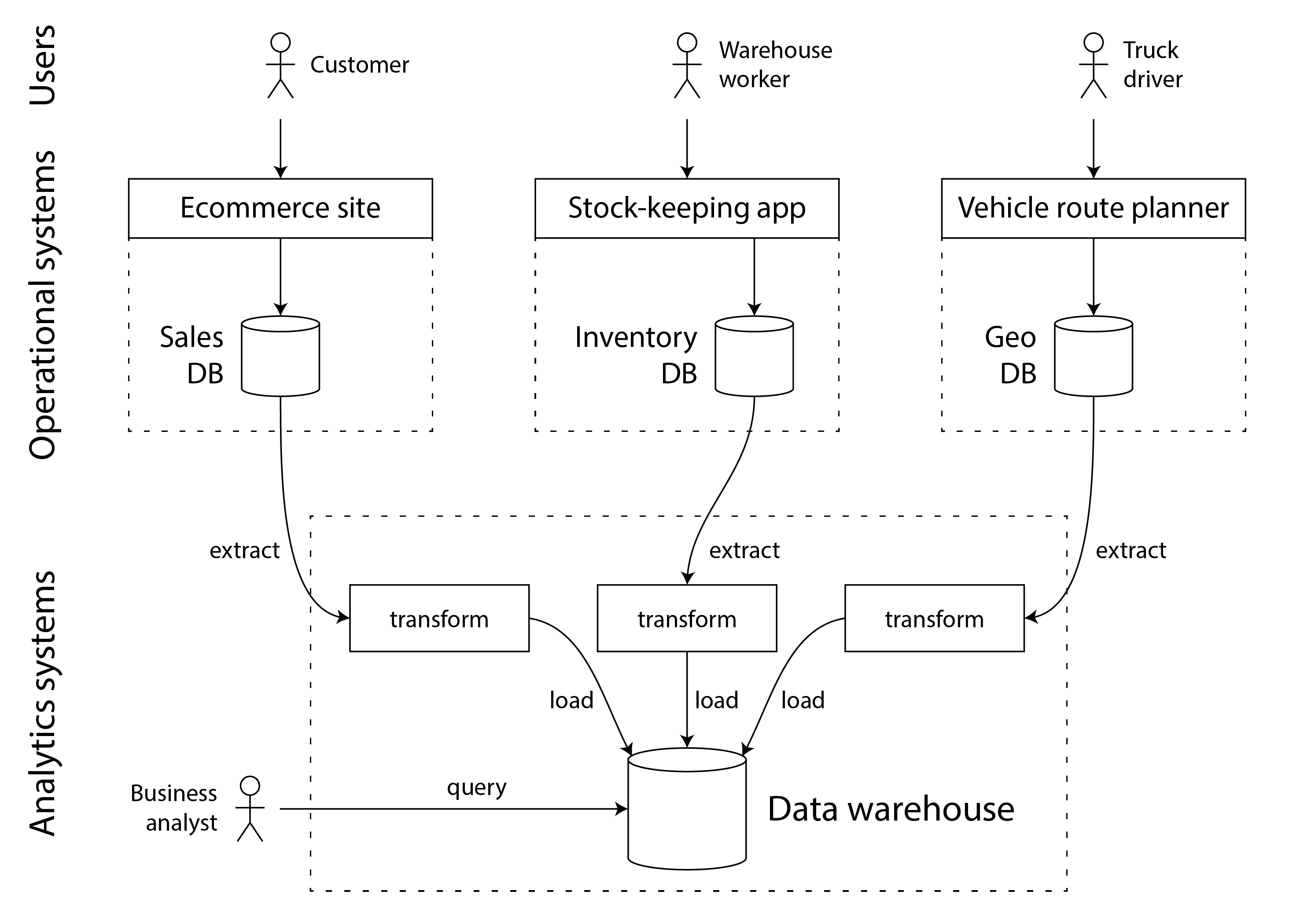
Figure 1-1 Simplified outline of ETL into a data warehouse.

In some cases the data sources of the ETL processes are external SaaS products such as customer relationship management (CRM), email marketing, or credit card processing systems. In those cases, you do not have direct access to the original database, since it is accessible only via the software vendor’s API. Bringing the data from these external systems into your own data warehouse can enable analyses that are not possible via the SaaS API. ETL for SaaS APIs is often implemented by specialist data connector services such as Fivetran, Singer, or AirByte.

Some database systems offer hybrid transactional/analytic processing (HTAP), which aims to enable OLTP and analytics in a single system without requiring ETL from one system into another ⁸ ⁹. However, many HTAP systems internally consist of an OLTP system coupled with a separate analytical system, hidden behind a common interface—so the distinction between the two remains important for understanding how these systems work.

Moreover, even though HTAP exists, it is common to have a separation between transactional and analytic systems due to their different goals and requirements. In particular, it is considered good practice for each operational system to have its own database (see “Microservices and Serverless”), leading to hundreds of separate operational databases; on the other hand, an enterprise usually has a single data warehouse, so that business analysts can combine data from several operational systems in a single query.

HTAP therefore does not replace data warehouses. Rather, it is useful in scenarios where the same application needs to both perform analytics queries that scan a large number of rows, and also read and update individual records with low latency. Fraud detection can involve such workloads, for example ¹⁰.

The separation between operational and analytical systems is part of a wider trend: as workloads have become more demanding, systems have become more specialized and optimized for particular workloads. General-purpose systems can handle small data volumes comfortably, but the greater the scale, the more specialized systems tend to become ¹¹.

From data warehouse to data lake

A data warehouse often uses a relational data model that is queried through SQL (see Chapter 3), perhaps using specialized business intelligence software. This model works well for the types of queries that business analysts need to make, but it is less well suited to the needs of data scientists, who might need to perform tasks such as:

Transform data into a form that is suitable for training a machine learning model; often this requires turning the rows and columns of a database table into a vector or matrix of numerical values called features. The process of performing this transformation in a way that maximizes the performance of the trained model is called feature engineering, and it often requires custom code that is difficult to express using SQL.
Take textual data (e.g., reviews of a product) and use natural language processing techniques to try to extract structured information from it (e.g., the sentiment of the author, or which topics they mention). Similarly, they might need to extract structured information from photos using computer vision techniques.

Although there have been efforts to add machine learning operators to a SQL data model ¹² and to build efficient machine learning systems on top of a relational foundation ¹³, many data scientists prefer not to work in a relational database such as a data warehouse. Instead, many prefer to use Python data analysis libraries such as pandas and scikit-learn, statistical analysis languages such as R, and distributed analytics frameworks such as Spark ¹⁴. We discuss these further in “Dataframes, Matrices, and Arrays”.

Consequently, organizations face a need to make data available in a form that is suitable for use by data scientists. The answer is a data lake: a centralized data repository that holds a copy of any data that might be useful for analysis, obtained from operational systems via ETL processes. The difference from a data warehouse is that a data lake simply contains files, without imposing any particular file format or data model. Files in a data lake might be collections of database records, encoded using a file format such as Avro or Parquet (see Chapter 5), but they can equally well contain text, images, videos, sensor readings, sparse matrices, feature vectors, genome sequences, or any other kind of data ¹⁵. Besides being more flexible, this is also often cheaper than relational data storage, since the data lake can use commoditized file storage such as object stores (see “Cloud-Native System Architecture”).

ETL processes have been generalized to data pipelines, and in some cases the data lake has become an intermediate stop on the path from the operational systems to the data warehouse. The data lake contains data in a “raw” form produced by the operational systems, without the transformation into a relational data warehouse schema. This approach has the advantage that each consumer of the data can transform the raw data into a form that best suits their needs. It has been dubbed the sushi principle: “raw data is better” ¹⁶.

Besides loading data from a data lake into a separate data warehouse, it is also possible to run typical data warehousing workloads (SQL queries and business analytics) directly on the files in the data lake, alongside data science/machine learning workloads. This architecture is known as a data lakehouse, and it requires a query execution engine and a metadata (e.g., schema management) layer that extend the data lake’s file storage ¹⁷.

Apache Hive, Spark SQL, Presto, and Trino are examples of this approach.

Beyond the data lake

As analytics practices have matured, organizations have been increasingly paying attention to the management and operations of analytics systems and data pipelines, as captured for example in the DataOps manifesto ¹⁸. Part of this are issues of governance, privacy, and compliance with regulation such as GDPR and CCPA, which we discuss in “Data Systems, Law, and Society” and “Legislation and Self-Regulation”.

Moreover, analytical data is increasingly made available not only as files and relational tables, but also as streams of events (see Chapter 12). With file-based data analysis you can re-run the analysis periodically (e.g., daily) in order to respond to changes in the data, but stream processing allows analytics systems to respond to events much faster, on the order of seconds. Depending on the application and how time-sensitive it is, a stream processing approach can be valuable, for example to identify and block potentially fraudulent or abusive activity.

In some cases the outputs of analytics systems are made available to operational systems (a process sometimes known as reverse ETL ¹⁹). For example, a machine-learning model that was trained on data in an analytics system may be deployed to production, so that it can generate recommendations for end-users, such as “people who bought X also bought Y”. Such deployed outputs of analytics systems are also known as data products ²⁰. Machine learning models can be deployed to operational systems using specialized tools such as TFX, Kubeflow, or MLflow.

Systems of Record and Derived Data

Related to the distinction between operational and analytical systems, this book also distinguishes between systems of record and derived data systems. These terms are useful because they can help you clarify the flow of data through a system:

Systems of record: A system of record, also known as source of truth, holds the authoritative or canonical version of some data. When new data comes in, e.g., as user input, it is first written here. Each fact is represented exactly once (the representation is typically normalized; see “Normalization, Denormalization, and Joins”). If there is any discrepancy between another system and the system of record, then the value in the system of record is (by definition) the correct one.
Derived data systems: Data in a derived system is the result of taking some existing data from another system and transforming or processing it in some way. If you lose derived data, you can recreate it from the original source. A classic example is a cache: data can be served from the cache if present, but if the cache doesn’t contain what you need, you can fall back to the underlying database. Denormalized values, indexes, materialized views, transformed data representations, and models trained on a dataset also fall into this category.

Technically speaking, derived data is redundant, in the sense that it duplicates existing information. However, it is often essential for getting good performance on read queries. You can derive several different datasets from a single source, enabling you to look at the data from different “points of view.”

Analytical systems are usually derived data systems, because they are consumers of data created elsewhere. Operational services may contain a mixture of systems of record and derived data systems. The systems of record are the primary databases to which data is first written, whereas the derived data systems are the indexes and caches that speed up common read operations, especially for queries that the system of record cannot answer efficiently.

Most databases, storage engines, and query languages are not inherently a system of record or a derived system. A database is just a tool: how you use it is up to you. The distinction between system of record and derived data system depends not on the tool, but on how you use it in your application. By being clear about which data is derived from which other data, you can bring clarity to an otherwise confusing system architecture.

When the data in one system is derived from the data in another, you need a process for updating the derived data when the original in the system of record changes. Unfortunately, many databases are designed based on the assumption that your application only ever needs to use that one database, and they do not make it easy to integrate multiple systems in order to propagate such updates. In “Data Integration” we will discuss approaches to data integration, which allow us to compose multiple data systems to achieve things that one system alone cannot do.

That brings us to the end of our comparison of analytics and transaction processing. In the next section, we will examine another trade-off that you might have already seen debated multiple times.

Cloud versus Self-Hosting

With anything that an organization needs to do, one of the first questions is: should it be done in-house, or should it be outsourced? Should you build or should you buy?

Ultimately, this is a question about business priorities. The received management wisdom is that things that are a core competency or a competitive advantage of your organization should be done in-house, whereas things that are non-core, routine, or commonplace should be left to a vendor ²¹. To give an extreme example, most companies do not generate their own electricity (unless they are an energy company, and leaving aside emergency backup power), since it is cheaper to buy electricity from the grid.

With software, two important decisions to be made are who builds the software and who deploys it. There is a spectrum of possibilities that outsource each decision to various degrees, as illustrated in Figure 1-2. At one extreme is bespoke software that you write and run in-house; at the other extreme are widely-used cloud services or Software as a Service (SaaS) products that are implemented and operated by an external vendor, and which you only access through a web interface or API.

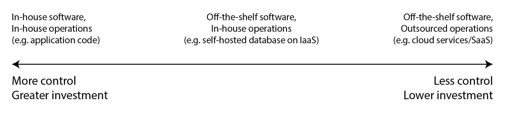
Figure 1-2 A spectrum of types of software and its operations.

The middle ground is off-the-shelf software (open source or commercial) that you self-host, i.e., deploy yourself—for example, if you download MySQL and install it on a server you control. This could be on your own hardware (often called on-premises, even if the server is actually in a rented datacenter rack and not literally on your own premises), or on a virtual machine in the cloud (Infrastructure as a Service or IaaS). There are still more points along this spectrum, e.g., taking open source software and running a modified version of it.

Separately from this spectrum there is also the question of how you deploy services, either in the cloud or on-premises—for example, whether you use an orchestration framework such as Kubernetes. However, choice of deployment tooling is out of scope of this book, since other factors have a greater influence on the architecture of data systems.

Pros and Cons of Cloud Services

Using a cloud service, rather than running comparable software yourself, essentially outsources the operation of that software to the cloud provider. There are good arguments for and against cloud services. Cloud providers claim that using their services saves you time and money, and allows you to move faster compared to setting up your own infrastructure.

Whether a cloud service is actually cheaper and easier than self-hosting depends very much on your skills and the workload on your systems. If you already have experience setting up and operating the systems you need, and if your load is quite predictable (i.e., the number of machines you need does not fluctuate wildly), then it’s often cheaper to buy your own machines and run the software on them yourself ²² ²³.

On the other hand, if you need a system that you don’t already know how to deploy and operate, then adopting a cloud service is often easier and quicker than learning to manage the system yourself. If you have to hire and train staff specifically to maintain and operate the system, that can get very expensive. You still need an operations team when you’re using the cloud (see “Operations in the Cloud Era”), but outsourcing the basic system administration can free up your team to focus on higher-level concerns.

When you outsource the operation of a system to a company that specializes in running that service, that can potentially result in a better service, since the provider gains operational expertise from providing the service to many customers. On the other hand, if you run the service yourself, you can configure and tune it to perform well on your particular workload; it is unlikely that a cloud service would be willing to make such customizations on your behalf.

Cloud services are particularly valuable if the load on your systems varies a lot over time. If you provision your machines to be able to handle peak load, but those computing resources are idle most of the time, the system becomes less cost-effective. In this situation, cloud services have the advantage that they can make it easier to scale your computing resources up or down in response to changes in demand.

For example, analytics systems often have extremely variable load: running a large analytical query quickly requires a lot of computing resources in parallel, but once the query completes, those resources sit idle until the user makes the next query. Predefined queries (e.g., for daily reports) can be enqueued and scheduled to smooth out the load, but for interactive queries, the faster you want them to complete, the more variable the workload becomes. If your dataset is so large that querying it quickly requires significant computing resources, using the cloud can save money, since you can return unused resources to the provider rather than leaving them idle. For smaller datasets, this difference is less significant.

The biggest downside of a cloud service is that you have no control over it:

If it is lacking a feature you need, all you can do is to politely ask the vendor whether they will add it; you generally cannot implement it yourself.
If the service goes down, all you can do is to wait for it to recover.
If you are using the service in a way that triggers a bug or causes performance problems, it will be difficult for you to diagnose the issue. With software that you run yourself, you can get performance metrics and debugging information from the operating system to help you understand its behavior, and you can look at the server logs, but with a service hosted by a vendor you usually do not have access to these internals.
Moreover, if the service shuts down or becomes unacceptably expensive, or if the vendor decides to change their product in a way you don’t like, you are at their mercy—continuing to run an old version of the software is usually not an option, so you will be forced to migrate to an alternative service ²⁴. This risk is mitigated if there are alternative services that expose a compatible API, but for many cloud services there are no standard APIs, which raises the cost of switching, making vendor lock-in a problem.
The cloud provider needs to be trusted to keep the data secure, which can complicate the process of complying with privacy and security regulations.

Despite all these risks, it has become more and more popular for organizations to build new applications on top of cloud services, or adopting a hybrid approach in which cloud services are used for some aspects of a system. However, cloud services will not subsume all in-house data systems: many older systems predate the cloud, and for any services that have specialist requirements that existing cloud services cannot meet, in-house systems remain necessary. For example, very latency-sensitive applications such as high-frequency trading require full control of the hardware.

Cloud-Native System Architecture

Besides having a different economic model (subscribing to a service instead of buying hardware and licensing software to run on it), the rise of the cloud has also had a profound effect on how data systems are implemented on a technical level. The term cloud-native is used to describe an architecture that is designed to take advantage of cloud services.

In principle, almost any software that you can self-host could also be provided as a cloud service, and indeed such managed services are now available for many popular data systems. However, systems that have been designed from the ground up to be cloud-native have been shown to have several advantages: better performance on the same hardware, faster recovery from failures, being able to quickly scale computing resources to match the load, and supporting larger datasets ²⁵ ²⁶ ²⁷. Table 1-2 lists some examples of both types of systems.

Category	Self-hosted systems	Cloud-native systems
Operational/OLTP	MySQL, PostgreSQL, MongoDB	AWS Aurora ²⁵, Azure SQL DB Hyperscale ²⁶, Google Cloud Spanner
Analytical/OLAP	Teradata, ClickHouse, Spark	Snowflake ²⁷, Google BigQuery, Azure Synapse Analytics

Table 1-2 Examples of self-hosted and cloud-native database systems

Layering of cloud services

Many self-hosted data systems have very simple system requirements: they run on a conventional operating system such as Linux or Windows, they store their data as files on the filesystem, and they communicate via standard network protocols such as TCP/IP. A few systems depend on special hardware such as GPUs (for machine learning) or RDMA network interfaces, but on the whole, self-hosted software tends to use very generic computing resources: CPU, RAM, a filesystem, and an IP network.

In a cloud, this type of software can be run on an Infrastructure-as-a-Service environment, using one or more virtual machines (or instances) with a certain allocation of CPUs, memory, disk, and network bandwidth. Compared to physical machines, cloud instances can be provisioned faster and they come in a greater variety of sizes, but otherwise they are similar to a traditional computer: you can run any software you like on it, but you are responsible for administering it yourself.

In contrast, the key idea of cloud-native services is to use not only the computing resources managed by your operating system, but also to build upon lower-level cloud services to create higher-level services. For example:

Object storage services such as Amazon S3, Azure Blob Storage, and Cloudflare R2 store large files. They provide more limited APIs than a typical filesystem (basic file reads and writes), but they have the advantage that they hide the underlying physical machines: the service automatically distributes the data across many machines, so that you don’t have to worry about running out of disk space on any one machine. Even if some machines or their disks fail entirely, no data is lost.
Many other services are in turn built upon object storage and other cloud services: for example, Snowflake is a cloud-based analytic database (data warehouse) that relies on S3 for data storage ²⁷, and some other services in turn build upon Snowflake.

As always with abstractions in computing, there is no one right answer to what you should use. As a general rule, higher-level abstractions tend to be more oriented towards particular use cases. If your needs match the situations for which a higher-level system is designed, using the existing higher-level system will probably provide what you need with much less hassle than building it yourself from lower-level systems. On the other hand, if there is no high-level system that meets your needs, then building it yourself from lower-level components is the only option.

Separation of storage and compute

In traditional computing, disk storage is regarded as durable (we assume that once something is written to disk, it will not be lost). To tolerate the failure of an individual hard disk, RAID (Redundant Array of Independent Disks) is often used to maintain copies of the data on several disks attached to the same machine. RAID can be performed either in hardware or in software by the operating system, and it is transparent to the applications accessing the filesystem.

In the cloud, compute instances (virtual machines) may also have local disks attached, but cloud-native systems typically treat these disks more like an ephemeral cache, and less like long-term storage. This is because the local disk becomes inaccessible if the associated instance fails, or if the instance is replaced with a bigger or a smaller one (on a different physical machine) in order to adapt to changes in load.

As an alternative to local disks, cloud services also offer virtual disk storage that can be detached from one instance and attached to a different one (Amazon EBS, Azure managed disks, and persistent disks in Google Cloud). Such a virtual disk is not actually a physical disk, but rather a cloud service provided by a separate set of machines, which emulates the behavior of a disk (a block device, where each block is typically 4 KiB in size). This technology makes it possible to run traditional disk-based software in the cloud, but the block device emulation introduces overheads that can be avoided in systems that are designed from the ground up for the cloud ²⁵. It also makes the application very sensitive to network glitches, since every I/O on the virtual block device is actually a network call ²⁸.

To address this problem, cloud-native services generally avoid using virtual disks, and instead build on dedicated storage services that are optimized for particular workloads. Object storage services such as S3 are designed for long-term storage of fairly large files, ranging from hundreds of kilobytes to several gigabytes in size. The individual rows or values stored in a database are typically much smaller than this; cloud databases therefore typically manage smaller values in a separate service, and store larger data blocks (containing many individual values) in an object store ²⁶ ²⁹. We will see ways of doing this in Chapter 4.

In a traditional systems architecture, the same computer is responsible for both storage (disk) and computation (CPU and RAM), but in cloud-native systems, these two responsibilities have become somewhat separated or disaggregated ⁹ ²⁷ ³⁰ ³¹: for example, S3 only stores files, and if you want to analyze that data, you will have to run the analysis code somewhere outside of S3. This implies transferring the data over the network, which we will discuss further in “Distributed versus Single-Node Systems”.

Moreover, cloud-native systems are often multitenant, which means that rather than having a separate machine for each customer, data and computation from several different customers are handled on the same shared hardware by the same service ³².

Multitenancy can enable better hardware utilization, easier scalability, and easier management by the cloud provider, but it also requires careful engineering to ensure that one customer’s activity does not affect the performance or security of the system for other customers ³³.

Operations in the Cloud Era

Traditionally, the people managing an organization’s server-side data infrastructure were known as database administrators (DBAs) or system administrators (sysadmins). More recently, many organizations have tried to integrate the roles of software development and operations into teams with a shared responsibility for both backend services and data infrastructure; the DevOps philosophy has guided this trend. Site Reliability Engineers (SREs) are Google’s implementation of this idea ³⁴.

The role of operations is to ensure services are reliably delivered to users (including configuring infrastructure and deploying applications), and to ensure a stable production environment (including monitoring and diagnosing any problems that may affect reliability). For self-hosted systems, operations traditionally involves a significant amount of work at the level of individual machines, such as capacity planning (e.g., monitoring available disk space and adding more disks before you run out of space), provisioning new machines, moving services from one machine to another, and installing operating system patches.

Many cloud services present an API that hides the individual machines that actually implement the service. For example, cloud storage replaces fixed-size disks with metered billing, where you can store data without planning your capacity needs in advance, and you are then charged based on the space actually used. Moreover, many cloud services remain highly available, even when individual machines have failed (see “Reliability and Fault Tolerance”).

This shift in emphasis from individual machines to services has been accompanied by a change in the role of operations. The high-level goal of providing a reliable service remains the same, but the processes and tools have evolved. The DevOps/SRE philosophy places greater emphasis on:

automation—preferring repeatable processes over manual one-off jobs,
preferring ephemeral virtual machines and services over long running servers,
enabling frequent application updates,
learning from incidents, and
preserving the organization’s knowledge about the system, even as individual people come and go ³⁵.

With the rise of cloud services, there has been a bifurcation of roles: operations teams at infrastructure companies specialize in the details of providing a reliable service to a large number of customers, while the customers of the service spend as little time and effort as possible on infrastructure ³⁶.

Customers of cloud services still require operations, but they focus on different aspects, such as choosing the most appropriate service for a given task, integrating different services with each other, and migrating from one service to another. Even though metered billing removes the need for capacity planning in the traditional sense, it’s still important to know what resources you are using for which purpose, so that you don’t waste money on cloud resources that are not needed: capacity planning becomes financial planning, and performance optimization becomes cost optimization ³⁷.

Moreover, cloud services do have resource limits or quotas (such as the maximum number of processes you can run concurrently), which you need to know about and plan for before you run into them ³⁸.

Adopting a cloud service can be easier and quicker than running your own infrastructure, although even here there is a cost in learning how to use it, and perhaps working around its limitations. Integration between different services becomes a particular challenge as a growing number of vendors offers an ever broader range of cloud services targeting different use cases ³⁹ ⁴⁰.

ETL (see “Data Warehousing”) is only part of the story; operational cloud services also need to be integrated with each other. At present, there is a lack of standards that would facilitate this sort of integration, so it often involves significant manual effort.

Other operational aspects that cannot fully be outsourced to cloud services include maintaining the security of an application and the libraries it uses, managing the interactions between your own services, monitoring the load on your services, and tracking down the cause of problems such as performance degradations or outages. While the cloud is changing the role of operations, the need for operations is as great as ever.

Distributed versus Single-Node Systems

A system that involves several machines communicating via a network is called a distributed system. Each of the processes participating in a distributed system is called a node. There are various reasons why you might want a system to be distributed:

Inherently distributed systems: If an application involves two or more interacting users, each using their own device, then the system is unavoidably distributed: the communication between the devices will have to go via a network.
Requests between cloud services: If data is stored in one service but processed in another, it must be transferred over the network from one service to the other.
Fault tolerance/high availability: If your application needs to continue working even if one machine (or several machines, or the network, or an entire datacenter) goes down, you can use multiple machines to give you redundancy. When one fails, another one can take over. See “Reliability and Fault Tolerance” and Chapter 6 on replication.
Scalability: If your data volume or computing requirements grow bigger than a single machine can handle, you can potentially spread the load across multiple machines. See “Scalability”.
Latency: If you have users around the world, you might want to have servers in various regions worldwide so that each user can be served from a server that is geographically close to them. That avoids the users having to wait for network packets to travel halfway around the world to answer their requests. See “Describing Performance”.
Elasticity: If your application is busy at some times and idle at other times, a cloud deployment can scale up or down to meet the demand, so that you pay only for resources you are actively using. This is more difficult on a single machine, which needs to be provisioned to handle the maximum load, even at times when it is barely used.
Using specialized hardware: Different parts of the system can take advantage of different types of hardware to match their workload. For example, an object store may use machines with many disks but few CPUs, whereas a data analysis system may use machines with lots of CPU and memory but no disks, and a machine learning system may use machines with GPUs (which are much more efficient than CPUs for training deep neural networks and other machine learning tasks).
Legal compliance: Some countries have data residency laws that require data about people in their jurisdiction to be stored and processed geographically within that country ⁴¹. The scope of these rules varies—for example, in some cases it applies only to medical or financial data, while other cases are broader. A service with users in several such jurisdictions will therefore have to distribute their data across servers in several locations.
Sustainability: If you have flexibility on where and when to run your jobs, you might be able to run them in a time and place where plenty of renewable electricity is available, and avoid running them when the power grid is under strain. This can reduce your carbon emissions and allow you to take advantage of cheap power when it is available ⁴² ⁴³.

These reasons apply both to services that you write yourself (application code) and services consisting of off-the-shelf software (such as databases).

Problems with Distributed Systems

Distributed systems also have downsides. Every request and API call that goes via the network needs to deal with the possibility of failure: the network may be interrupted, or the service may be overloaded or crashed, and therefore any request may time out without receiving a response. In this case, we don’t know whether the service received the request, and simply retrying it might not be safe. We will discuss these problems in detail in Chapter 9.

Although datacenter networks are fast, making a call to another service is still vastly slower than calling a function in the same process ⁴⁴.

When operating on large volumes of data, rather than transferring the data from storage to a separate machine that processes it, it can be faster to bring the computation to the machine that already has the data ⁴⁵.

More nodes are not always faster: in some cases, a simple single-threaded program on one computer can perform significantly better than a cluster with over 100 CPU cores ⁴⁶.

Troubleshooting a distributed system is often difficult: if the system is slow to respond, how do you figure out where the problem lies? Techniques for diagnosing problems in distributed systems are developed under the heading of observability ⁴⁷ ⁴⁸, which involves collecting data about the execution of a system, and allowing it to be queried in ways that allows both high-level metrics and individual events to be analyzed. Tracing tools such as OpenTelemetry, Zipkin, and Jaeger allow you to track which client called which server for which operation, and how long each call took ⁴⁹.

Databases provide various mechanisms for ensuring data consistency, as we shall see in Chapter 6 and Chapter 8. However, when each service has its own database, maintaining consistency of data across those different services becomes the application’s problem. Distributed transactions, which we explore in Chapter 8, are a possible technique for ensuring consistency, but they are rarely used in a microservices context because they run counter to the goal of making services independent from each other, and many databases don’t support them ⁵⁰.

For all these reasons, if you can do something on a single machine, this is often much simpler and cheaper compared to setting up a distributed system ²³ ⁴⁶ ⁵¹. CPUs, memory, and disks have grown larger, faster, and more reliable. When combined with single-node databases such as DuckDB, SQLite, and KùzuDB, many workloads can now run on a single node. We will explore more on this topic in Chapter 4.

Microservices and Serverless

The most common way of distributing a system across multiple machines is to divide them into clients and servers, and let the clients make requests to the servers. Most commonly HTTP is used for this communication, as we will discuss in “Dataflow Through Services: REST and RPC”. The same process may be both a server (handling incoming requests) and a client (making outbound requests to other services).

This way of building applications has traditionally been called a service-oriented architecture (SOA); more recently the idea has been refined into a microservices architecture ⁵² ⁵³. In this architecture, a service has one well-defined purpose (for example, in the case of S3, this would be file storage); each service exposes an API that can be called by clients via the network, and each service has one team that is responsible for its maintenance. A complex application can thus be decomposed into multiple interacting services, each managed by a separate team.

There are several advantages to breaking down a complex piece of software into multiple services: each service can be updated independently, reducing coordination effort among teams; each service can be assigned the hardware resources it needs; and by hiding the implementation details behind an API, the service owners are free to change the implementation without affecting clients. In terms of data storage, it is common for each service to have its own databases, and not to share databases between services: sharing a database would effectively make the entire database structure a part of the service’s API, and then that structure would be difficult to change. Shared databases could also cause one service’s queries to negatively impact the performance of other services.

On the other hand, having many services can itself breed complexity: each service requires infrastructure for deploying new releases, adjusting the allocated hardware resources to match the load, collecting logs, monitoring service health, and alerting an on-call engineer in the case of a problem. Orchestration frameworks such as Kubernetes have become a popular way of deploying services, since they provide a foundation for this infrastructure. Testing a service during development can be complicated, since you also need to run all the other services that it depends on.

Microservice APIs can be challenging to evolve. Clients that call an API expect the API to have certain fields. Developers might wish to add or remove fields to an API as business needs change, but doing so can cause clients to fail. Worse still, such failures are often not discovered until late in the development cycle when the updated service API is deployed to a staging or production environment. API description standards such as OpenAPI and gRPC help manage the relationship between client and server APIs; we discuss these further in Chapter 5.

Microservices are primarily a technical solution to a people problem: allowing different teams to make progress independently without having to coordinate with each other. This is valuable in a large company, but in a small company where there are not many teams, using microservices is likely to be unnecessary overhead, and it is preferable to implement the application in the simplest way possible ⁵².

Serverless, or function-as-a-service (FaaS), is another approach to deploying services, in which the management of the infrastructure is outsourced to a cloud vendor ³³. When using virtual machines, you have to explicitly choose when to start up or shut down an instance; in contrast, with the serverless model, the cloud provider automatically allocates and frees hardware resources as needed, based on the incoming requests to your service ⁵⁴. Serverless deployment shifts more of the operational burden to cloud providers and enables flexible billing by usage rather than machine instances. To offer such benefits, many serverless infrastructure providers impose a time limit on function execution, limit runtime environments, and might suffer from slow start times when a function is first invoked. The term “serverless” can also be misleading: each serverless function execution still runs on a server, but subsequent executions might run on a different one. Moreover, infrastructure such as BigQuery and various Kafka offerings have adopted “serverless” terminology to signal that their services auto-scale and that they bill by usage rather than machine instances.

Just like cloud storage replaced capacity planning (deciding in advance how many disks to buy) with a metered billing model, the serverless approach is bringing metered billing to code execution: you only pay for the time that your application code is actually running, rather than having to provision resources in advance.

Cloud Computing versus Supercomputing

Cloud computing is not the only way of building large-scale computing systems; an alternative is high-performance computing (HPC), also known as supercomputing. Although there are overlaps, HPC often has different priorities and uses different techniques compared to cloud computing and enterprise datacenter systems. Some of those differences are:

Supercomputers are typically used for computationally intensive scientific computing tasks, such as weather forecasting, climate modeling, molecular dynamics (simulating the movement of atoms and molecules), complex optimization problems, and solving partial differential equations. On the other hand, cloud computing tends to be used for online services, business data systems, and similar systems that need to serve user requests with high availability.
A supercomputer typically runs large batch jobs that checkpoint the state of their computation to disk from time to time. If a node fails, a common solution is to simply stop the entire cluster workload, repair the faulty node, and then restart the computation from the last checkpoint ⁵⁵ ⁵⁶. With cloud services, it is usually not desirable to stop the entire cluster, since the services need to continually serve users with minimal interruptions.
Supercomputer nodes typically communicate through shared memory and remote direct memory access (RDMA), which support high bandwidth and low latency, but assume a high level of trust among the users of the system ⁵⁷. In cloud computing, the network and the machines are often shared by mutually untrusting organizations, requiring stronger security mechanisms such as resource isolation (e.g., virtual machines), encryption and authentication.
Cloud datacenter networks are often based on IP and Ethernet, arranged in Clos topologies to provide high bisection bandwidth—a commonly used measure of a network’s overall performance ⁵⁵ ⁵⁸. Supercomputers often use specialized network topologies, such as multi-dimensional meshes and toruses ⁵⁹, which yield better performance for HPC workloads with known communication patterns.
Cloud computing allows nodes to be distributed across multiple geographic regions, whereas supercomputers generally assume that all of their nodes are close together.

Large-scale analytics systems sometimes share some characteristics with supercomputing, which is why it can be worth knowing about these techniques if you are working in this area. However, this book is mostly concerned with services that need to be continually available, as discussed in “Reliability and Fault Tolerance”.

Data Systems, Law, and Society

So far you’ve seen in this chapter that the architecture of data systems is influenced not only by technical goals and requirements, but also by the human needs of the organizations that they support. Increasingly, data systems engineers are realizing that serving the needs of their own business is not enough: we also have a responsibility towards society at large.

One particular concern are systems that store data about people and their behavior. Since 2018 the General Data Protection Regulation (GDPR) has given residents of many European countries greater control and legal rights over their personal data, and similar privacy regulation has been adopted in various other countries and states around the world, including for example the California Consumer Privacy Act (CCPA). Regulations around AI, such as the EU AI Act, place further restrictions on how personal data can be used.

Moreover, even in areas that are not directly subject to regulation, there is increasing recognition of the effects that computer systems have on people and society. Social media has changed how individuals consume news, which influences their political opinions and hence may affect the outcome of elections. Automated systems increasingly make decisions that have profound consequences for individuals, such as deciding who should be given a loan or insurance coverage, who should be invited to a job interview, or who should be suspected of a crime ⁶⁰.

Everyone who works on such systems shares a responsibility for considering the ethical impact and ensuring that they comply with relevant law. It is not necessary for everybody to become an expert in law and ethics, but a basic awareness of legal and ethical principles is just as important as, say, some foundational knowledge in distributed systems.

Legal considerations are influencing the very foundations of how data systems are being designed ⁶¹. For example, the GDPR grants individuals the right to have their data erased on request (sometimes known as the right to be forgotten). However, as we shall see in this book, many data systems rely on immutable constructs such as append-only logs as part of their design; how can we ensure deletion of some data in the middle of a file that is supposed to be immutable? How do we handle deletion of data that has been incorporated into derived datasets (see “Systems of Record and Derived Data”), such as training data for machine learning models? Answering these questions creates new engineering challenges.

At present we don’t have clear guidelines on which particular technologies or system architectures should be considered “GDPR-compliant” or not. The regulation deliberately does not mandate particular technologies, because these may quickly change as technology progresses. Instead, the legal texts set out high-level principles that are subject to interpretation. This means that there are no simple answers to the question of how to comply with privacy regulation, but we will look at some of the technologies in this book through this lens.

In general, we store data because we think that its value is greater than the costs of storing it. However, it is worth remembering that the costs of storage are not just the bill you pay for Amazon S3 or another service: the cost-benefit calculation should also take into account the risks of liability and reputational damage if the data were to be leaked or compromised by adversaries, and the risk of legal costs and fines if the storage and processing of the data is found not to be compliant with the law ⁵¹.

Governments or police forces might also compel companies to hand over data. When there is a risk that the data may reveal criminalized behaviors (for example, homosexuality in several Middle Eastern and African countries, or seeking an abortion in several US states), storing that data creates real safety risks for users. Travel to an abortion clinic, for example, could easily be revealed by location data, perhaps even by a log of the user’s IP addresses over time (which indicate approximate location).

Once all the risks are taken into account, it might be reasonable to decide that some data is simply not worth storing, and that it should therefore be deleted. This principle of data minimization (sometimes known by the German term Datensparsamkeit) runs counter to the “big data” philosophy of storing lots of data speculatively in case it turns out to be useful in the future ⁶². But it fits with the GDPR, which mandates that personal data may only be collected for a specified, explicit purpose, that this data may not later be used for any other purpose, and that the data must not be kept for longer than necessary for the purposes for which it was collected ⁶³.

Businesses have also taken notice of privacy and safety concerns. Credit card companies require payment processing businesses to adhere to strict payment card industry (PCI) standards. Processors undergo frequent evaluations from independent auditors to verify continued compliance. Software vendors have also seen increased scrutiny. Many buyers now require their vendors to comply with Service Organization Control (SOC) Type 2 standards. As with PCI compliance, vendors undergo third party audits to verify adherence.

Generally, it is important to balance the needs of your business against the needs of the people whose data you are collecting and processing. There is much more to this topic; in Chapter 14 we will go deeper into the topics of ethics and legal compliance, including the problems of bias and discrimination.

Summary

The theme of this chapter has been to understand trade-offs: that is, to recognize that for many questions there is not one right answer, but several different approaches that each have various pros and cons. We explored some of the most important choices that affect the architecture of data systems, and introduced terminology that will be needed throughout the rest of this book.

We started by making a distinction between operational (transaction-processing, OLTP) and analytical (OLAP) systems, and saw their different characteristics: not only managing different types of data with different access patterns, but also serving different audiences. We encountered the concept of a data warehouse and data lake, which receive data feeds from operational systems via ETL. In Chapter 4 we will see that operational and analytical systems often use very different internal data layouts because of the different types of queries they need to serve.

We then compared cloud services, a comparatively recent development, to the traditional paradigm of self-hosted software that has previously dominated data systems architecture. Which of these approaches is more cost-effective depends a lot on your particular situation, but it’s undeniable that cloud-native approaches are bringing big changes to the way data systems are architected, for example in the way they separate storage and compute.

Cloud systems are intrinsically distributed, and we briefly examined some of the trade-offs of distributed systems compared to using a single machine. There are situations in which you can’t avoid going distributed, but it’s advisable not to rush into making a system distributed if it’s possible to keep it on a single machine. In Chapter 9 we will cover the challenges with distributed systems in more detail.

Finally, we saw that data systems architecture is determined not only by the needs of the business deploying the system, but also by privacy regulation that protects the rights of the people whose data is being processed—an aspect that many engineers are prone to ignoring. How we translate legal requirements into technical implementations is not yet well understood, but it’s important to keep this question in mind as we move through the rest of this book.

References

Richard T. Kouzes, Gordon A. Anderson, Stephen T. Elbert, Ian Gorton, and Deborah K. Gracio. The Changing Paradigm of Data-Intensive Computing. IEEE Computer, volume 42, issue 1, January 2009. doi:10.1109/MC.2009.26 ↩︎
Martin Kleppmann, Adam Wiggins, Peter van Hardenberg, and Mark McGranaghan. Local-first software: you own your data, in spite of the cloud. At 2019 ACM SIGPLAN International Symposium on New Ideas, New Paradigms, and Reflections on Programming and Software (Onward!), October 2019. doi:10.1145/3359591.3359737 ↩︎
Joe Reis and Matt Housley. Fundamentals of Data Engineering. O’Reilly Media, 2022. ISBN: 9781098108304 ↩︎
Rui Pedro Machado and Helder Russa. Analytics Engineering with SQL and dbt. O’Reilly Media, 2023. ISBN: 9781098142384 ↩︎
Edgar F. Codd, S. B. Codd, and C. T. Salley. Providing OLAP to User-Analysts: An IT Mandate. E. F. Codd Associates, 1993. Archived at perma.cc/RKX8-2GEE ↩︎
Chinmay Soman and Neha Pawar. Comparing Three Real-Time OLAP Databases: Apache Pinot, Apache Druid, and ClickHouse. startree.ai, April 2023. Archived at perma.cc/8BZP-VWPA ↩︎
Surajit Chaudhuri and Umeshwar Dayal. An Overview of Data Warehousing and OLAP Technology. ACM SIGMOD Record, volume 26, issue 1, pages 65–74, March 1997. doi:10.1145/248603.248616 ↩︎
Fatma Özcan, Yuanyuan Tian, and Pinar Tözün. Hybrid Transactional/Analytical Processing: A Survey. At ACM International Conference on Management of Data (SIGMOD), May 2017. doi:10.1145/3035918.3054784 ↩︎
Adam Prout, Szu-Po Wang, Joseph Victor, Zhou Sun, Yongzhu Li, Jack Chen, Evan Bergeron, Eric Hanson, Robert Walzer, Rodrigo Gomes, and Nikita Shamgunov. Cloud-Native Transactions and Analytics in SingleStore. At International Conference on Management of Data (SIGMOD), June 2022. doi:10.1145/3514221.3526055 ↩︎ ↩︎
Chao Zhang, Guoliang Li, Jintao Zhang, Xinning Zhang, and Jianhua Feng. HTAP Databases: A Survey. IEEE Transactions on Knowledge and Data Engineering, April 2024. doi:10.1109/TKDE.2024.3389693 ↩︎
Michael Stonebraker and Uğur Çetintemel. ‘One Size Fits All’: An Idea Whose Time Has Come and Gone. At 21st International Conference on Data Engineering (ICDE), April 2005. doi:10.1109/ICDE.2005.1 ↩︎
Jeffrey Cohen, Brian Dolan, Mark Dunlap, Joseph M. Hellerstein, and Caleb Welton. MAD Skills: New Analysis Practices for Big Data. Proceedings of the VLDB Endowment, volume 2, issue 2, pages 1481–1492, August 2009. doi:10.14778/1687553.1687576 ↩︎
Dan Olteanu. The Relational Data Borg is Learning. Proceedings of the VLDB Endowment, volume 13, issue 12, August 2020. doi:10.14778/3415478.3415572 ↩︎
Matt Bornstein, Martin Casado, and Jennifer Li. Emerging Architectures for Modern Data Infrastructure: 2020. future.a16z.com, October 2020. Archived at perma.cc/LF8W-KDCC ↩︎
Martin Fowler. DataLake. martinfowler.com, February 2015. Archived at perma.cc/4WKN-CZUK ↩︎
Bobby Johnson and Joseph Adler. The Sushi Principle: Raw Data Is Better. At Strata+Hadoop World, February 2015. ↩︎
Michael Armbrust, Ali Ghodsi, Reynold Xin, and Matei Zaharia. Lakehouse: A New Generation of Open Platforms that Unify Data Warehousing and Advanced Analytics. At 11th Annual Conference on Innovative Data Systems Research (CIDR), January 2021. ↩︎
DataKitchen, Inc. The DataOps Manifesto. dataopsmanifesto.org, 2017. Archived at perma.cc/3F5N-FUQ4 ↩︎
Tejas Manohar. What is Reverse ETL: A Definition & Why It’s Taking Off. hightouch.io, November 2021. Archived at perma.cc/A7TN-GLYJ ↩︎
Simon O’Regan. Designing Data Products. towardsdatascience.com, August 2018. Archived at perma.cc/HU67-3RV8 ↩︎
Camille Fournier. Why is it so hard to decide to buy? skamille.medium.com, July 2021. Archived at perma.cc/6VSG-HQ5X ↩︎
David Heinemeier Hansson. Why we’re leaving the cloud. world.hey.com, October 2022. Archived at perma.cc/82E6-UJ65 ↩︎
Nima Badizadegan. Use One Big Server. specbranch.com, August 2022. Archived at perma.cc/M8NB-95UK ↩︎ ↩︎
Steve Yegge. Dear Google Cloud: Your Deprecation Policy is Killing You. steve-yegge.medium.com, August 2020. Archived at perma.cc/KQP9-SPGU ↩︎
Alexandre Verbitski, Anurag Gupta, Debanjan Saha, Murali Brahmadesam, Kamal Gupta, Raman Mittal, Sailesh Krishnamurthy, Sandor Maurice, Tengiz Kharatishvili, and Xiaofeng Bao. Amazon Aurora: Design Considerations for High Throughput Cloud-Native Relational Databases. At ACM International Conference on Management of Data (SIGMOD), pages 1041–1052, May 2017. doi:10.1145/3035918.3056101 ↩︎ ↩︎ ↩︎
Panagiotis Antonopoulos, Alex Budovski, Cristian Diaconu, Alejandro Hernandez Saenz, Jack Hu, Hanuma Kodavalla, Donald Kossmann, Sandeep Lingam, Umar Farooq Minhas, Naveen Prakash, Vijendra Purohit, Hugh Qu, Chaitanya Sreenivas Ravella, Krystyna Reisteter, Sheetal Shrotri, Dixin Tang, and Vikram Wakade. Socrates: The New SQL Server in the Cloud. At ACM International Conference on Management of Data (SIGMOD), pages 1743–1756, June 2019. doi:10.1145/3299869.3314047 ↩︎ ↩︎ ↩︎
Midhul Vuppalapati, Justin Miron, Rachit Agarwal, Dan Truong, Ashish Motivala, and Thierry Cruanes. Building An Elastic Query Engine on Disaggregated Storage. At 17th USENIX Symposium on Networked Systems Design and Implementation (NSDI), February 2020. ↩︎ ↩︎ ↩︎ ↩︎
Nick Van Wiggeren. The Real Failure Rate of EBS. planetscale.com, March 2025. Archived at perma.cc/43CR-SAH5 ↩︎
Colin Breck. Predicting the Future of Distributed Systems. blog.colinbreck.com, August 2024. Archived at perma.cc/K5FC-4XX2 ↩︎
Gwen Shapira. Compute-Storage Separation Explained. thenile.dev, January 2023. Archived at perma.cc/QCV3-XJNZ ↩︎
Ravi Murthy and Gurmeet Goindi. AlloyDB for PostgreSQL under the hood: Intelligent, database-aware storage. cloud.google.com, May 2022. Archived at archive.org ↩︎
Jack Vanlightly. The Architecture of Serverless Data Systems. jack-vanlightly.com, November 2023. Archived at perma.cc/UDV4-TNJ5 ↩︎
Eric Jonas, Johann Schleier-Smith, Vikram Sreekanti, Chia-Che Tsai, Anurag Khandelwal, Qifan Pu, Vaishaal Shankar, Joao Carreira, Karl Krauth, Neeraja Yadwadkar, Joseph E. Gonzalez, Raluca Ada Popa, Ion Stoica, David A. Patterson. Cloud Programming Simplified: A Berkeley View on Serverless Computing. arxiv.org, February 2019. ↩︎ ↩︎
Betsy Beyer, Jennifer Petoff, Chris Jones, and Niall Richard Murphy. Site Reliability Engineering: How Google Runs Production Systems. O’Reilly Media, 2016. ISBN: 9781491929124 ↩︎
Thomas Limoncelli. The Time I Stole $10,000 from Bell Labs. ACM Queue, volume 18, issue 5, November 2020. doi:10.1145/3434571.3434773 ↩︎
Charity Majors. The Future of Ops Jobs. acloudguru.com, August 2020. Archived at perma.cc/GRU2-CZG3 ↩︎
Boris Cherkasky. (Over)Pay As You Go for Your Datastore. medium.com, September 2021. Archived at perma.cc/Q8TV-2AM2 ↩︎
Shlomi Kushchi. Serverless Doesn’t Mean DevOpsLess or NoOps. thenewstack.io, February 2023. Archived at perma.cc/3NJR-AYYU ↩︎
Erik Bernhardsson. Storm in the stratosphere: how the cloud will be reshuffled. erikbern.com, November 2021. Archived at perma.cc/SYB2-99P3 ↩︎
Benn Stancil. The data OS. benn.substack.com, September 2021. Archived at perma.cc/WQ43-FHS6 ↩︎
Maria Korolov. Data residency laws pushing companies toward residency as a service. csoonline.com, January 2022. Archived at perma.cc/CHE4-XZZ2 ↩︎
Severin Borenstein. Can Data Centers Flex Their Power Demand? energyathaas.wordpress.com, April 2025. Archived at https://perma.cc/MUD3-A6FF ↩︎
Bilge Acun, Benjamin Lee, Fiodar Kazhamiaka, Aditya Sundarrajan, Kiwan Maeng, Manoj Chakkaravarthy, David Brooks, and Carole-Jean Wu. Carbon Dependencies in Datacenter Design and Management. ACM SIGENERGY Energy Informatics Review, volume 3, issue 3, pages 21–26. doi:10.1145/3630614.3630619 ↩︎
Kousik Nath. These are the numbers every computer engineer should know. freecodecamp.org, September 2019. Archived at perma.cc/RW73-36RL ↩︎
Joseph M. Hellerstein, Jose Faleiro, Joseph E. Gonzalez, Johann Schleier-Smith, Vikram Sreekanti, Alexey Tumanov, and Chenggang Wu. Serverless Computing: One Step Forward, Two Steps Back. At Conference on Innovative Data Systems Research (CIDR), January 2019. ↩︎
Frank McSherry, Michael Isard, and Derek G. Murray. Scalability! But at What COST? At 15th USENIX Workshop on Hot Topics in Operating Systems (HotOS), May 2015. ↩︎ ↩︎
Cindy Sridharan. Distributed Systems Observability: A Guide to Building Robust Systems. Report, O’Reilly Media, May 2018. Archived at perma.cc/M6JL-XKCM ↩︎
Charity Majors. Observability — A 3-Year Retrospective. thenewstack.io, August 2019. Archived at perma.cc/CG62-TJWL ↩︎
Benjamin H. Sigelman, Luiz André Barroso, Mike Burrows, Pat Stephenson, Manoj Plakal, Donald Beaver, Saul Jaspan, and Chandan Shanbhag. Dapper, a Large-Scale Distributed Systems Tracing Infrastructure. Google Technical Report dapper-2010-1, April 2010. Archived at perma.cc/K7KU-2TMH ↩︎
Rodrigo Laigner, Yongluan Zhou, Marcos Antonio Vaz Salles, Yijian Liu, and Marcos Kalinowski. Data management in microservices: State of the practice, challenges, and research directions. Proceedings of the VLDB Endowment, volume 14, issue 13, pages 3348–3361, September 2021. doi:10.14778/3484224.3484232 ↩︎
Jordan Tigani. Big Data is Dead. motherduck.com, February 2023. Archived at perma.cc/HT4Q-K77U ↩︎ ↩︎
Sam Newman. Building Microservices, second edition. O’Reilly Media, 2021. ISBN: 9781492034025 ↩︎ ↩︎
Chris Richardson. Microservices: Decomposing Applications for Deployability and Scalability. infoq.com, May 2014. Archived at perma.cc/CKN4-YEQ2 ↩︎
Mohammad Shahrad, Rodrigo Fonseca, Íñigo Goiri, Gohar Chaudhry, Paul Batum, Jason Cooke, Eduardo Laureano, Colby Tresness, Mark Russinovich, Ricardo Bianchini. Serverless in the Wild: Characterizing and Optimizing the Serverless Workload at a Large Cloud Provider. At USENIX Annual Technical Conference (ATC), July 2020. ↩︎
Luiz André Barroso, Urs Hölzle, and Parthasarathy Ranganathan. The Datacenter as a Computer: Designing Warehouse-Scale Machines, third edition. Morgan & Claypool Synthesis Lectures on Computer Architecture, October 2018. doi:10.2200/S00874ED3V01Y201809CAC046 ↩︎ ↩︎
David Fiala, Frank Mueller, Christian Engelmann, Rolf Riesen, Kurt Ferreira, and Ron Brightwell. Detection and Correction of Silent Data Corruption for Large-Scale High-Performance Computing,” at International Conference for High Performance Computing, Networking, Storage and Analysis (SC), November 2012. doi:10.1109/SC.2012.49 ↩︎
Anna Kornfeld Simpson, Adriana Szekeres, Jacob Nelson, and Irene Zhang. Securing RDMA for High-Performance Datacenter Storage Systems. At 12th USENIX Workshop on Hot Topics in Cloud Computing (HotCloud), July 2020. ↩︎
Arjun Singh, Joon Ong, Amit Agarwal, Glen Anderson, Ashby Armistead, Roy Bannon, Seb Boving, Gaurav Desai, Bob Felderman, Paulie Germano, Anand Kanagala, Jeff Provost, Jason Simmons, Eiichi Tanda, Jim Wanderer, Urs Hölzle, Stephen Stuart, and Amin Vahdat. Jupiter Rising: A Decade of Clos Topologies and Centralized Control in Google’s Datacenter Network. At Annual Conference of the ACM Special Interest Group on Data Communication (SIGCOMM), August 2015. doi:10.1145/2785956.2787508 ↩︎
Glenn K. Lockwood. Hadoop’s Uncomfortable Fit in HPC. glennklockwood.blogspot.co.uk, May 2014. Archived at perma.cc/S8XX-Y67B ↩︎
Cathy O’Neil: Weapons of Math Destruction: How Big Data Increases Inequality and Threatens Democracy. Crown Publishing, 2016. ISBN: 9780553418811 ↩︎
Supreeth Shastri, Vinay Banakar, Melissa Wasserman, Arun Kumar, and Vijay Chidambaram. Understanding and Benchmarking the Impact of GDPR on Database Systems. Proceedings of the VLDB Endowment, volume 13, issue 7, pages 1064–1077, March 2020. doi:10.14778/3384345.3384354 ↩︎
Martin Fowler. Datensparsamkeit. martinfowler.com, December 2013. Archived at perma.cc/R9QX-CME6 ↩︎
Regulation (EU) 2016/679 of the European Parliament and of the Council of 27 April 2016 (General Data Protection Regulation). Official Journal of the European Union L 119/1, May 2016. ↩︎

2. Defining Nonfunctional Requirements

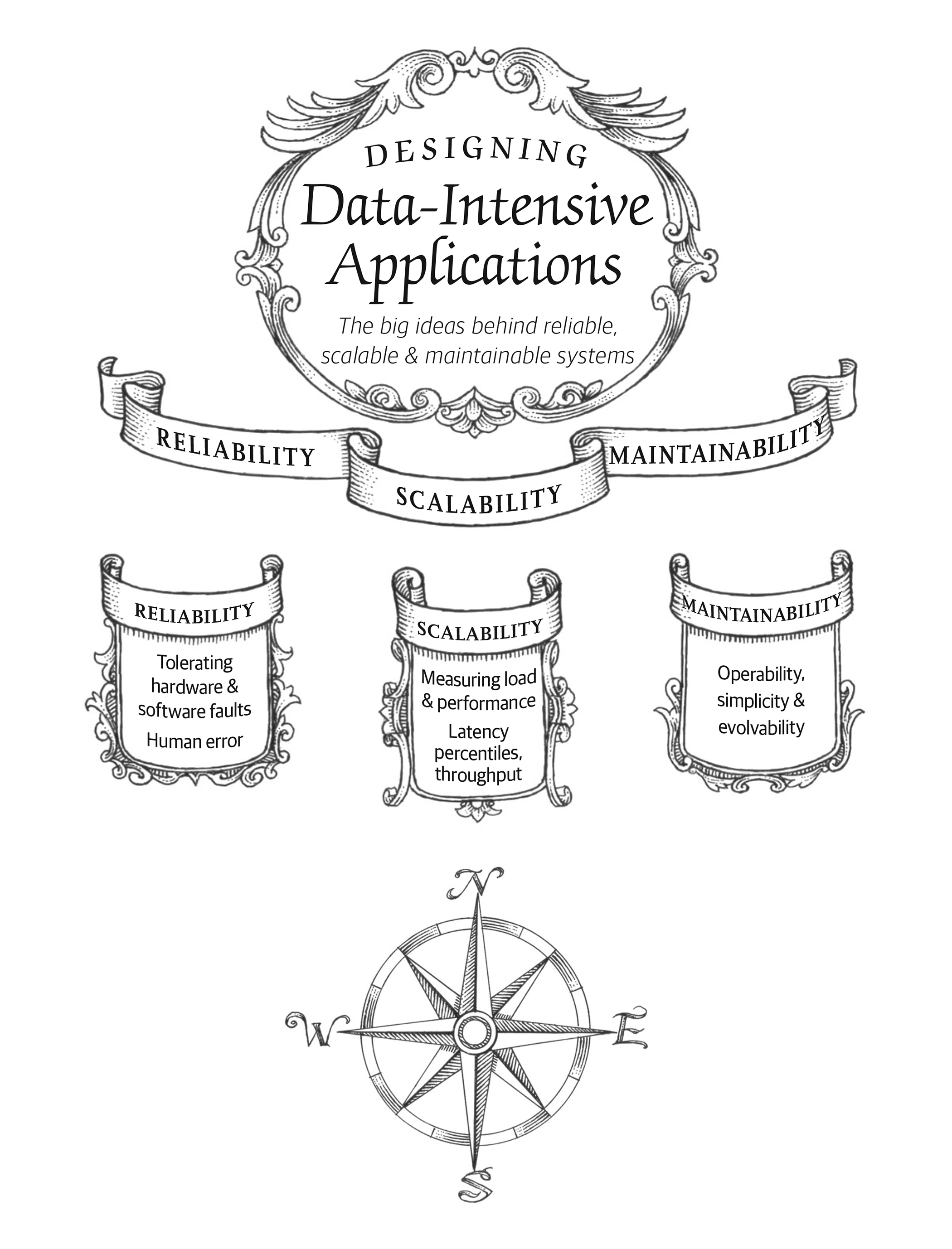
The Internet was done so well that most people think of it as a natural resource like the Pacific Ocean, rather than something that was man-made. When was the last time a technology with a scale like that was so error-free?

Alan Kay, in interview with Dr Dobb’s Journal (2012)

If you are building an application, you will be driven by a list of requirements. At the top of your list is most likely the functionality that the application must offer: what screens and what buttons you need, and what each operation is supposed to do in order to fulfill the purpose of your software. These are your functional requirements.

In addition, you probably also have some nonfunctional requirements: for example, the app should be fast, reliable, secure, legally compliant, and easy to maintain. These requirements might not be explicitly written down, because they may seem somewhat obvious, but they are just as important as the app’s functionality: an app that is unbearably slow or unreliable might as well not exist.

Many nonfunctional requirements, such as security, fall outside the scope of this book. But there are a few nonfunctional requirements that we will consider, and this chapter will help you articulate them for your own systems:

How to define and measure the performance of a system (see “Describing Performance”);
What it means for a service to be reliable—namely, continuing to work correctly, even when things go wrong (see “Reliability and Fault Tolerance”);
Allowing a system to be scalable by having efficient ways of adding computing capacity as the load on the system grows (see “Scalability”); and
Making it easier to maintain a system in the long term (see “Maintainability”).

The terminology introduced in this chapter will also be useful in the following chapters, when we go into the details of how data-intensive systems are implemented. However, abstract definitions can be quite dry; to make the ideas more concrete, we will start this chapter with a case study of how a social networking service might work, which will provide practical examples of performance and scalability.

Case Study: Social Network Home Timelines

Imagine you are given the task of implementing a social network in the style of X (formerly Twitter), in which users can post messages and follow other users. This will be a huge simplification of how such a service actually works ¹ ² ³, but it will help illustrate some of the issues that arise in large-scale systems.

Let’s assume that users make 500 million posts per day, or 5,700 posts per second on average. Occasionally, the rate can spike as high as 150,000 posts/second ⁴. Let’s also assume that the average user follows 200 people and has 200 followers (although there is a very wide range: most people have only a handful of followers, and a few celebrities such as Barack Obama have over 100 million followers).

Representing Users, Posts, and Follows

Imagine we keep all of the data in a relational database as shown in Figure 2-1. We have one table for users, one table for posts, and one table for follow relationships.

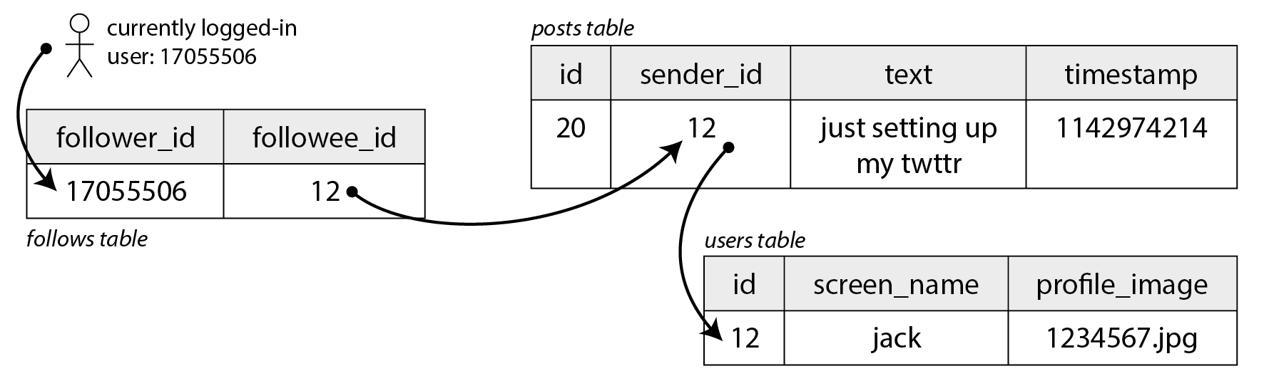
Figure 2-1 Simple relational schema for a social network in which users can follow each other.

Let’s say the main read operation that our social network must support is the home timeline, which displays recent posts by people you are following (for simplicity we will ignore ads, suggested posts from people you are not following, and other extensions). We could write the following SQL query to get the home timeline for a particular user:

SELECT posts.*, users.* FROM posts
    JOIN follows ON posts.sender_id = follows.followee_id
    JOIN users ON posts.sender_id = users.id
    WHERE follows.follower_id = current_user
    ORDER BY posts.timestamp DESC
    LIMIT 1000

To execute this query, the database will use the follows table to find everybody who current_user is following, look up recent posts by those users, and sort them by timestamp to get the most recent 1,000 posts by any of the followed users.

Posts are supposed to be timely, so let’s assume that after somebody makes a post, we want their followers to be able to see it within 5 seconds. One way of doing that would be for the user’s client to repeat the query above every 5 seconds while the user is online (this is known as polling). If we assume that 10 million users are online and logged in at the same time, that would mean running the query 2 million times per second. Even if you increase the polling interval, this is a lot.

Moreover, the query above is quite expensive: if you are following 200 people, it needs to fetch a list of recent posts by each of those 200 people, and merge those lists. 2 million timeline queries per second then means that the database needs to look up the recent posts from some sender 400 million times per second—a huge number. And that is the average case. Some users follow tens of thousands of accounts; for them, this query is very expensive to execute, and difficult to make fast.

Materializing and Updating Timelines

How can we do better? Firstly, instead of polling, it would be better if the server actively pushed new posts to any followers who are currently online. Secondly, we should precompute the results of the query above so that a user’s request for their home timeline can be served from a cache.

Imagine that for each user we store a data structure containing their home timeline, i.e., the recent posts by people they are following. Every time a user makes a post, we look up all of their followers, and insert that post into the home timeline of each follower—like delivering a message to a mailbox. Now when a user logs in, we can simply give them this home timeline that we precomputed. Moreover, to receive a notification about any new posts on their timeline, the user’s client simply needs to subscribe to the stream of posts being added to their home timeline.

The downside of this approach is that we now need to do more work every time a user makes a post, because the home timelines are derived data that needs to be updated. The process is illustrated in Figure 2-2. When one initial request results in several downstream requests being carried out, we use the term fan-out to describe the factor by which the number of requests increases.

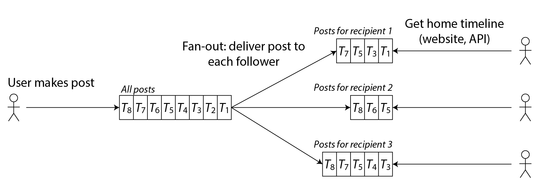
Figure 2-2 Fan-out: delivering new posts to every follower of the user who made the post.

At a rate of 5,700 posts posted per second, if the average post reaches 200 followers (i.e., a fan-out factor of 200), we will need to do just over 1 million home timeline writes per second. This is a lot, but it’s still a significant saving compared to the 400 million per-sender post lookups per second that we would otherwise have to do.

If the rate of posts spikes due to some special event, we don’t have to do the timeline deliveries immediately—we can enqueue them and accept that it will temporarily take a bit longer for posts to show up in followers’ timelines. Even during such load spikes, timelines remain fast to load, since we simply serve them from a cache.

This process of precomputing and updating the results of a query is called materialization, and the timeline cache is an example of a materialized view (a concept we will discuss further in “Maintaining materialized views”). The materialized view speeds up reads, but in return we have to do more work on write. The cost of writes for most users is modest, but a social network also has to consider some extreme cases:

If a user is following a very large number of accounts, and those accounts post a lot, that user will have a high rate of writes to their materialized timeline. However, in this case it’s unlikely that the user is actually reading all of the posts in their timeline, and therefore it’s okay to simply drop some of their timeline writes and show the user only a sample of the posts from the accounts they’re following ⁵.
When a celebrity account with a very large number of followers makes a post, we have to do a large amount of work to insert that post into the home timelines of each of their millions of followers. In this case it’s not okay to drop some of those writes. One way of solving this problem is to handle celebrity posts separately from everyone else’s posts: we can save ourselves the effort of adding them to millions of timelines by storing the celebrity posts separately and merging them with the materialized timeline when it is read. Despite such optimizations, handling celebrities on a social network can require a lot of infrastructure ⁶.

Describing Performance

Most discussions of software performance consider two main types of metric:

Response time: The elapsed time from the moment when a user makes a request until they receive the requested answer. The unit of measurement is seconds (or milliseconds, or microseconds).
Throughput: The number of requests per second, or the data volume per second, that the system is processing. For a given allocation of hardware resources, there is a maximum throughput that can be handled. The unit of measurement is “somethings per second”.

In the social network case study, “posts per second” and “timeline writes per second” are throughput metrics, whereas the “time it takes to load the home timeline” or the “time until a post is delivered to followers” are response time metrics.

There is often a connection between throughput and response time; an example of such a relationship for an online service is sketched in Figure 2-3. The service has a low response time when request throughput is low, but response time increases as load increases. This is because of queueing: when a request arrives on a highly loaded system, it’s likely that the CPU is already in the process of handling an earlier request, and therefore the incoming request needs to wait until the earlier request has been completed. As throughput approaches the maximum that the hardware can handle, queueing delays increase sharply.

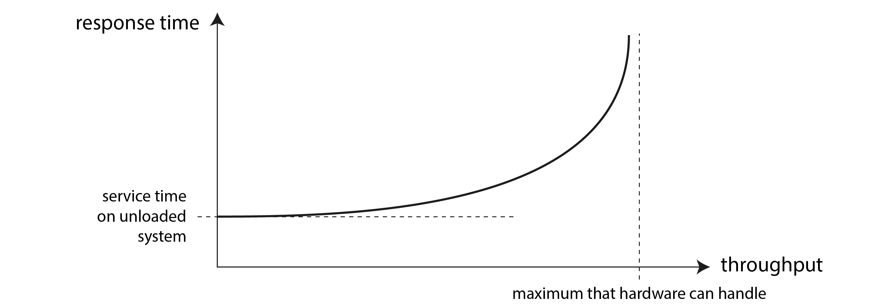
Figure 2-3 As the throughput of a service approaches its capacity, the response time increases dramatically due to queueing.

WHEN AN OVERLOADED SYSTEM WON’T RECOVER

If a system is close to overload, with throughput pushed close to the limit, it can sometimes enter a vicious cycle where it becomes less efficient and hence even more overloaded. For example, if there is a long queue of requests waiting to be handled, response times may increase so much that clients time out and resend their request. This causes the rate of requests to increase even further, making the problem worse—a retry storm. Even when the load is reduced again, such a system may remain in an overloaded state until it is rebooted or otherwise reset. This phenomenon is called a metastable failure, and it can cause serious outages in production systems ⁷ ⁸.

To avoid retries overloading a service, you can increase and randomize the time between successive retries on the client side (exponential backoff ⁹ ¹⁰), and temporarily stop sending requests to a service that has returned errors or timed out recently (using a circuit breaker ¹¹ ¹² or token bucket algorithm ¹³). The server can also detect when it is approaching overload and start proactively rejecting requests (load shedding ¹⁴), and send back responses asking clients to slow down (backpressure ¹ ¹⁵). The choice of queueing and load-balancing algorithms can also make a difference ¹⁶.

In terms of performance metrics, the response time is usually what users care about the most, whereas the throughput determines the required computing resources (e.g., how many servers you need), and hence the cost of serving a particular workload. If throughput is likely to increase beyond what the current hardware can handle, the capacity needs to be expanded; a system is said to be scalable if its maximum throughput can be significantly increased by adding computing resources.

In this section we will focus primarily on response times, and we will return to throughput and scalability in “Scalability”.

Latency and Response Time

“Latency” and “response time” are sometimes used interchangeably, but in this book we will use the terms in a specific way (illustrated in Figure 2-4):

The response time is what the client sees; it includes all delays incurred anywhere in the system.
The service time is the duration for which the service is actively processing the user request.
Queueing delays can occur at several points in the flow: for example, after a request is received, it might need to wait until a CPU is available before it can be processed; a response packet might need to be buffered before it is sent over the network if other tasks on the same machine are sending a lot of data via the outbound network interface.
Latency is a catch-all term for time during which a request is not being actively processed, i.e., during which it is latent. In particular, network latency or network delay refers to the time that request and response spend traveling through the network.

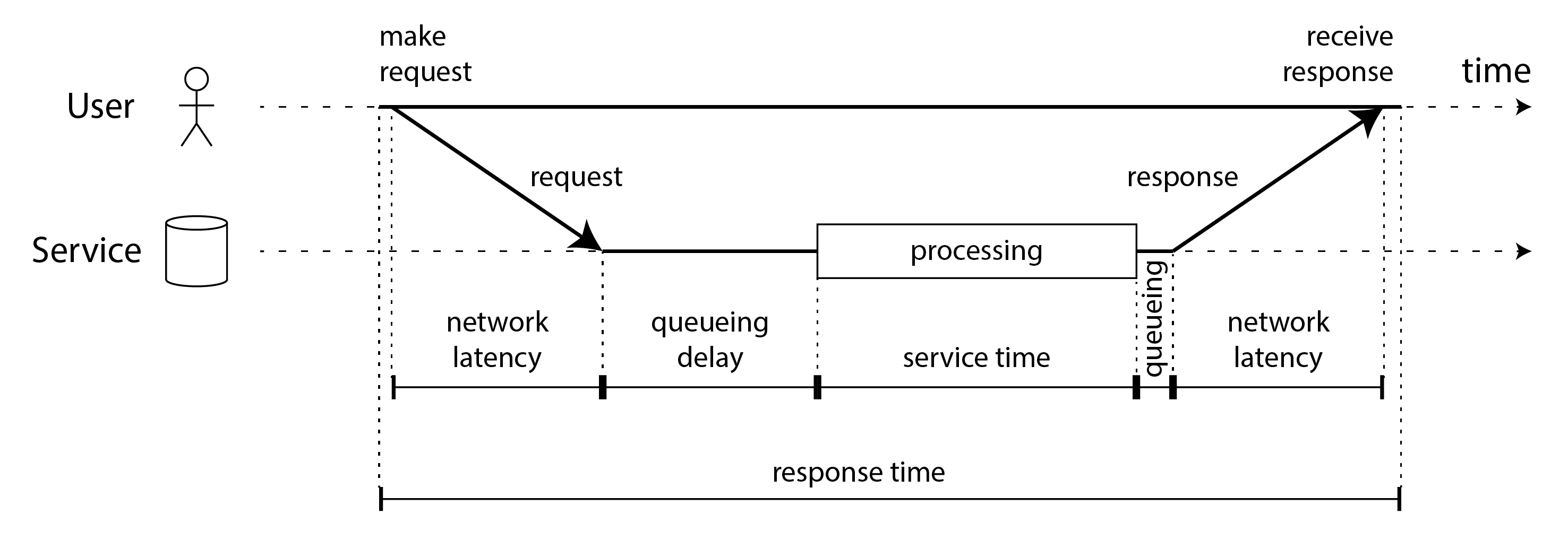
Figure 2-4 Response time, service time, network latency, and queueing delay.

In Figure 2-4, time flows from left to right, each communicating node is shown as a horizontal line, and a request or response message is shown as a thick diagonal arrow from one node to another. You will encounter this style of diagram frequently over the course of this book.

The response time can vary significantly from one request to the next, even if you keep making the same request over and over again. Many factors can add random delays: for example, a context switch to a background process, the loss of a network packet and TCP retransmission, a garbage collection pause, a page fault forcing a read from disk, mechanical vibrations in the server rack ¹⁷, or many other causes. We will discuss this topic in more detail in “Timeouts and Unbounded Delays”.

Queueing delays often account for a large part of the variability in response times. As a server can only process a small number of things in parallel (limited, for example, by its number of CPU cores), it only takes a small number of slow requests to hold up the processing of subsequent requests—an effect known as head-of-line blocking. Even if those subsequent requests have fast service times, the client will see a slow overall response time due to the time waiting for the prior request to complete. The queueing delay is not part of the service time, and for this reason it is important to measure response times on the client side.

Average, Median, and Percentiles

Because the response time varies from one request to the next, we need to think of it not as a single number, but as a distribution of values that you can measure. In Figure 2-5, each gray bar represents a request to a service, and its height shows how long that request took. Most requests are reasonably fast, but there are occasional outliers that take much longer. Variation in network delay is also known as jitter.

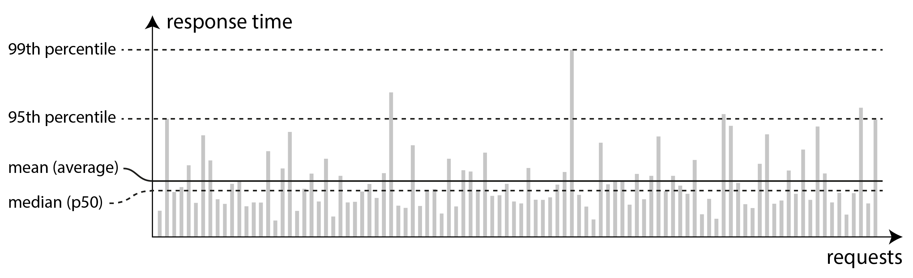
Figure 2-5 Illustrating mean and percentiles: response times for a sample of 100 requests to a service.

It’s common to report the average response time of a service (technically, the arithmetic mean: that is, sum all the response times, and divide by the number of requests). The mean response time is useful for estimating throughput limits ¹⁸. However, the mean is not a very good metric if you want to know your “typical” response time, because it doesn’t tell you how many users actually experienced that delay.

Usually it is better to use percentiles. If you take your list of response times and sort it from fastest to slowest, then the median is the halfway point: for example, if your median response time is 200 ms, that means half your requests return in less than 200 ms, and half your requests take longer than that. This makes the median a good metric if you want to know how long users typically have to wait. The median is also known as the 50th percentile, and sometimes abbreviated as p50.

In order to figure out how bad your outliers are, you can look at higher percentiles: the 95th, 99th, and 99.9th percentiles are common (abbreviated p95, p99, and p999). They are the response time thresholds at which 95%, 99%, or 99.9% of requests are faster than that particular threshold. For example, if the 95th percentile response time is 1.5 seconds, that means 95 out of 100 requests take less than 1.5 seconds, and 5 out of 100 requests take 1.5 seconds or more. This is illustrated in Figure 2-5.

High percentiles of response times, also known as tail latencies, are important because they directly affect users’ experience of the service. For example, Amazon describes response time requirements for internal services in terms of the 99.9th percentile, even though it only affects 1 in 1,000 requests. This is because the customers with the slowest requests are often those who have the most data on their accounts because they have made many purchases—that is, they’re the most valuable customers ¹⁹. It’s important to keep those customers happy by ensuring the website is fast for them.

On the other hand, optimizing the 99.99th percentile (the slowest 1 in 10,000 requests) was deemed too expensive and to not yield enough benefit for Amazon’s purposes. Reducing response times at very high percentiles is difficult because they are easily affected by random events outside of your control, and the benefits are diminishing.

THE USER IMPACT OF RESPONSE TIMES

It seems intuitively obvious that a fast service is better for users than a slow service ²⁰. However, it is surprisingly difficult to get hold of reliable data to quantify the effect that latency has on user behavior.

Some often-cited statistics are unreliable. In 2006 Google reported that a slowdown in search results from 400 ms to 900 ms was associated with a 20% drop in traffic and revenue ²¹. However, another Google study from 2009 reported that a 400 ms increase in latency resulted in only 0.6% fewer searches per day ²², and in the same year Bing found that a two-second increase in load time reduced ad revenue by 4.3% ²³. Newer data from these companies appears not to be publicly available.

A more recent Akamai study ²⁴ claims that a 100 ms increase in response time reduced the conversion rate of e-commerce sites by up to 7%; however, on closer inspection, the same study reveals that very fast page load times are also correlated with lower conversion rates! This seemingly paradoxical result is explained by the fact that the pages that load fastest are often those that have no useful content (e.g., 404 error pages). However, since the study makes no effort to separate the effects of page content from the effects of load time, its results are probably not meaningful.

A study by Yahoo ²⁵ compares click-through rates on fast-loading versus slow-loading search results, controlling for quality of search results. It finds 20–30% more clicks on fast searches when the difference between fast and slow responses is 1.25 seconds or more.

Use of Response Time Metrics

High percentiles are especially important in backend services that are called multiple times as part of serving a single end-user request. Even if you make the calls in parallel, the end-user request still needs to wait for the slowest of the parallel calls to complete. It takes just one slow call to make the entire end-user request slow, as illustrated in Figure 2-6. Even if only a small percentage of backend calls are slow, the chance of getting a slow call increases if an end-user request requires multiple backend calls, and so a higher proportion of end-user requests end up being slow (an effect known as tail latency amplification ²⁶).

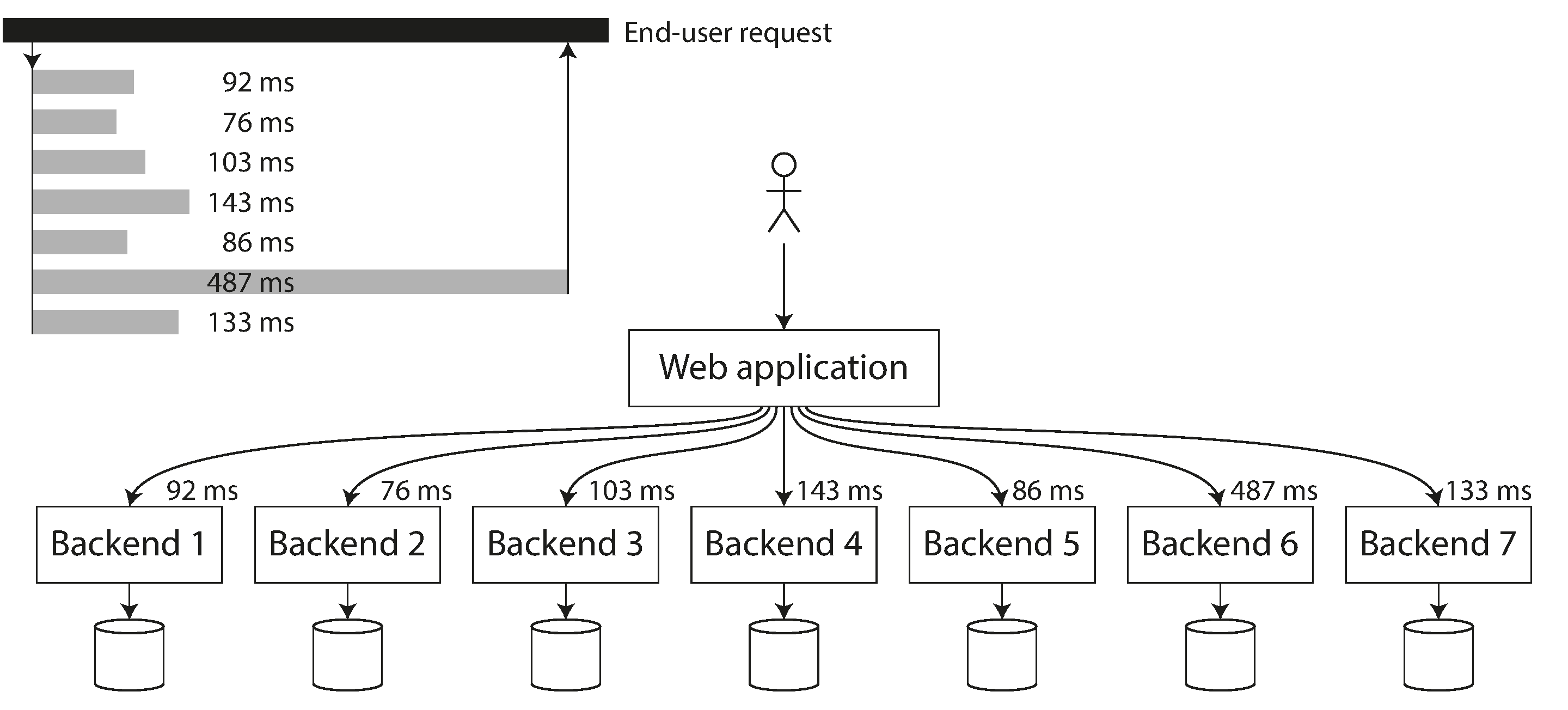
Figure 2-6 When several backend calls are needed to serve a request, it takes just a single slow backend request to slow down the entire end-user request.

Percentiles are often used in service level objectives (SLOs) and service level agreements (SLAs) as ways of defining the expected performance and availability of a service ²⁷. For example, an SLO may set a target for a service to have a median response time of less than 200 ms and a 99th percentile under 1 s, and a target that at least 99.9% of valid requests result in non-error responses. An SLA is a contract that specifies what happens if the SLO is not met (for example, customers may be entitled to a refund). That is the basic idea, at least; in practice, defining good availability metrics for SLOs and SLAs is not straightforward ²⁸ ²⁹.

COMPUTING PERCENTILES

If you want to add response time percentiles to the monitoring dashboards for your services, you need to efficiently calculate them on an ongoing basis. For example, you may want to keep a rolling window of response times of requests in the last 10 minutes. Every minute, you calculate the median and various percentiles over the values in that window and plot those metrics on a graph.

The simplest implementation is to keep a list of response times for all requests within the time window and to sort that list every minute. If that is too inefficient for you, there are algorithms that can calculate a good approximation of percentiles at minimal CPU and memory cost. Open source percentile estimation libraries include HdrHistogram, t-digest ³⁰ ³¹, OpenHistogram ³², and DDSketch ³³.

Beware that averaging percentiles, e.g., to reduce the time resolution or to combine data from several machines, is mathematically meaningless—the right way of aggregating response time data is to add the histograms ³⁴.

Reliability and Fault Tolerance

Everybody has an intuitive idea of what it means for something to be reliable or unreliable. For software, typical expectations include:

The application performs the function that the user expected.
It can tolerate the user making mistakes or using the software in unexpected ways.
Its performance is good enough for the required use case, under the expected load and data volume.
The system prevents any unauthorized access and abuse.

If all those things together mean “working correctly,” then we can understand reliability as meaning, roughly, “continuing to work correctly, even when things go wrong.” To be more precise about things going wrong, we will distinguish between faults and failures ³⁵ ³⁶ ³⁷:

Fault: A fault is when a particular part of a system stops working correctly: for example, if a single hard drive malfunctions, or a single machine crashes, or an external service (that the system depends on) has an outage.
Failure: A failure is when the system as a whole stops providing the required service to the user; in other words, when it does not meet the service level objective (SLO).

The distinction between fault and failure can be confusing because they are the same thing, just at different levels. For example, if a hard drive stops working, we say that the hard drive has failed: if the system consists only of that one hard drive, it has stopped providing the required service. However, if the system you’re talking about contains many hard drives, then the failure of a single hard drive is only a fault from the point of view of the bigger system, and the bigger system might be able to tolerate that fault by having a copy of the data on another hard drive.

Fault Tolerance

We call a system fault-tolerant if it continues providing the required service to the user in spite of certain faults occurring. If a system cannot tolerate a certain part becoming faulty, we call that part a single point of failure (SPOF), because a fault in that part escalates to cause the failure of the whole system.

For example, in the social network case study, a fault that might happen is that during the fan-out process, a machine involved in updating the materialized timelines crashes or become unavailable. To make this process fault-tolerant, we would need to ensure that another machine can take over this task without missing any posts that should have been delivered, and without duplicating any posts. (This idea is known as exactly-once semantics, and we will examine it in detail in “The End-to-End Argument for Databases”.)

Fault tolerance is always limited to a certain number of certain types of faults. For example, a system might be able to tolerate a maximum of two hard drives failing at the same time, or a maximum of one out of three nodes crashing. It would not make sense to tolerate any number of faults: if all nodes crash, there is nothing that can be done. If the entire planet Earth (and all servers on it) were swallowed by a black hole, tolerance of that fault would require web hosting in space—good luck getting that budget item approved.

Counter-intuitively, in such fault-tolerant systems, it can make sense to increase the rate of faults by triggering them deliberately—for example, by randomly killing individual processes without warning. This is called fault injection. Many critical bugs are actually due to poor error handling ³⁸; by deliberately inducing faults, you ensure that the fault-tolerance machinery is continually exercised and tested, which can increase your confidence that faults will be handled correctly when they occur naturally. Chaos engineering is a discipline that aims to improve confidence in fault-tolerance mechanisms through experiments such as deliberately injecting faults ³⁹.

Although we generally prefer tolerating faults over preventing faults, there are cases where prevention is better than cure (e.g., because no cure exists). This is the case with security matters, for example: if an attacker has compromised a system and gained access to sensitive data, that event cannot be undone. However, this book mostly deals with the kinds of faults that can be cured, as described in the following sections.

Hardware and Software Faults

When we think of causes of system failure, hardware faults quickly come to mind:

Approximately 2–5% of magnetic hard drives fail per year ⁴⁰ ⁴¹; in a storage cluster with 10,000 disks, we should therefore expect on average one disk failure per day. Recent data suggests that disks are getting more reliable, but failure rates remain significant ⁴².
Approximately 0.5–1% of solid state drives (SSDs) fail per year ⁴³. Small numbers of bit errors are corrected automatically ⁴⁴, but uncorrectable errors occur approximately once per year per drive, even in drives that are fairly new (i.e., that have experienced little wear); this error rate is higher than that of magnetic hard drives ⁴⁵, ⁴⁶.
Other hardware components such as power supplies, RAID controllers, and memory modules also fail, although less frequently than hard drives ⁴⁷ ⁴⁸.
Approximately one in 1,000 machines has a CPU core that occasionally computes the wrong result, likely due to manufacturing defects ⁴⁹ ⁵⁰ ⁵¹. In some cases, an erroneous computation leads to a crash, but in other cases it leads to a program simply returning the wrong result.
Data in RAM can also be corrupted, either due to random events such as cosmic rays, or due to permanent physical defects. Even when memory with error-correcting codes (ECC) is used, more than 1% of machines encounter an uncorrectable error in a given year, which typically leads to a crash of the machine and the affected memory module needing to be replaced ⁵². Moreover, certain pathological memory access patterns can flip bits with high probability ⁵³.
An entire datacenter might become unavailable (for example, due to power outage or network misconfiguration) or even be permanently destroyed (for example by fire, flood, or earthquake ⁵⁴). A solar storm, which induces large electrical currents in long-distance wires when the sun ejects a large mass of charged particles, could damage power grids and undersea network cables ⁵⁵. Although such large-scale failures are rare, their impact can be catastrophic if a service cannot tolerate the loss of a datacenter ⁵⁶.

These events are rare enough that you often don’t need to worry about them when working on a small system, as long as you can easily replace hardware that becomes faulty. However, in a large-scale system, hardware faults happen often enough that they become part of the normal system operation.

Tolerating hardware faults through redundancy

Our first response to unreliable hardware is usually to add redundancy to the individual hardware components in order to reduce the failure rate of the system. Disks may be set up in a RAID configuration (spreading data across multiple disks in the same machine so that a failed disk does not cause data loss), servers may have dual power supplies and hot-swappable CPUs, and datacenters may have batteries and diesel generators for backup power. Such redundancy can often keep a machine running uninterrupted for years.

Redundancy is most effective when component faults are independent, that is, the occurrence of one fault does not change how likely it is that another fault will occur. However, experience has shown that there are often significant correlations between component failures ⁴¹ ⁵⁷ ⁵⁸; unavailability of an entire server rack or an entire datacenter still happens more often than we would like.

Hardware redundancy increases the uptime of a single machine; however, as discussed in “Distributed versus Single-Node Systems”, there are advantages to using a distributed system, such as being able to tolerate a complete outage of one datacenter. For this reason, cloud systems tend to focus less on the reliability of individual machines, and instead aim to make services highly available by tolerating faulty nodes at the software level. Cloud providers use availability zones to identify which resources are physically co-located; resources in the same place are more likely to fail at the same time than geographically separated resources.

The fault-tolerance techniques we discuss in this book are designed to tolerate the loss of entire machines, racks, or availability zones. They generally work by allowing a machine in one datacenter to take over when a machine in another datacenter fails or becomes unreachable. We will discuss such techniques for fault tolerance in Chapter 6, Chapter 10, and at various other points in this book.

Systems that can tolerate the loss of entire machines also have operational advantages: a single-server system requires planned downtime if you need to reboot the machine (to apply operating system security patches, for example), whereas a multi-node fault-tolerant system can be patched by restarting one node at a time, without affecting the service for users. This is called a rolling upgrade, and we will discuss it further in Chapter 5.

Software faults

Although hardware failures can be weakly correlated, they are still mostly independent: for example, if one disk fails, it’s likely that other disks in the same machine will be fine for another while. On the other hand, software faults are often very highly correlated, because it is common for many nodes to run the same software and thus have the same bugs ⁵⁹ ⁶⁰. Such faults are harder to anticipate, and they tend to cause many more system failures than uncorrelated hardware faults ⁴⁷. For example:

A software bug that causes every node to fail at the same time in particular circumstances. For example, on June 30, 2012, a leap second caused many Java applications to hang simultaneously due to a bug in the Linux kernel, bringing down many Internet services ⁶¹. Due to a firmware bug, all SSDs of certain models suddenly fail after precisely 32,768 hours of operation (less than 4 years), rendering the data on them unrecoverable ⁶².
A runaway process that uses up some shared, limited resource, such as CPU time, memory, disk space, network bandwidth, or threads ⁶³. For example, a process that consumes too much memory while processing a large request may be killed by the operating system. A bug in a client library could cause a much higher request volume than anticipated ⁶⁴.
A service that the system depends on slows down, becomes unresponsive, or starts returning corrupted responses.
An interaction between different systems results in emergent behavior that does not occur when each system was tested in isolation ⁶⁵.
Cascading failures, where a problem in one component causes another component to become overloaded and slow down, which in turn brings down another component ⁶⁶ ⁶⁷.

The bugs that cause these kinds of software faults often lie dormant for a long time until they are triggered by an unusual set of circumstances. In those circumstances, it is revealed that the software is making some kind of assumption about its environment—and while that assumption is usually true, it eventually stops being true for some reason ⁶⁸ ⁶⁹.

There is no quick solution to the problem of systematic faults in software. Lots of small things can help: carefully thinking about assumptions and interactions in the system; thorough testing; process isolation; allowing processes to crash and restart; avoiding feedback loops such as retry storms (see “When an overloaded system won’t recover”); measuring, monitoring, and analyzing system behavior in production.

Humans and Reliability

Humans design and build software systems, and the operators who keep the systems running are also human. Unlike machines, humans don’t just follow rules; their strength is being creative and adaptive in getting their job done. However, this characteristic also leads to unpredictability, and sometimes mistakes that can lead to failures, despite best intentions. For example, one study of large internet services found that configuration changes by operators were the leading cause of outages, whereas hardware faults (servers or network) played a role in only 10–25% of outages ⁷⁰.

It is tempting to label such problems as “human error” and to wish that they could be solved by better controlling human behavior through tighter procedures and compliance with rules. However, blaming people for mistakes is counterproductive. What we call “human error” is not really the cause of an incident, but rather a symptom of a problem with the sociotechnical system in which people are trying their best to do their jobs ⁷¹. Often complex systems have emergent behavior, in which unexpected interactions between components may also lead to failures ⁷².

Various technical measures can help minimize the impact of human mistakes, including thorough testing (both hand-written tests and property testing on lots of random inputs) ³⁸, rollback mechanisms for quickly reverting configuration changes, gradual roll-outs of new code, detailed and clear monitoring, observability tools for diagnosing production issues (see “Problems with Distributed Systems”), and well-designed interfaces that encourage “the right thing” and discourage “the wrong thing”.

However, these things require an investment of time and money, and in the pragmatic reality of everyday business, organizations often prioritize revenue-generating activities over measures that increase their resilience against mistakes. If there is a choice between more features and more testing, many organizations understandably choose features. Given this choice, when a preventable mistake inevitably occurs, it does not make sense to blame the person who made the mistake—the problem is the organization’s priorities.

Increasingly, organizations are adopting a culture of blameless postmortems: after an incident, the people involved are encouraged to share full details about what happened, without fear of punishment, since this allows others in the organization to learn how to prevent similar problems in the future ⁷³. This process may uncover a need to change business priorities, a need to invest in areas that have been neglected, a need to change the incentives for the people involved, or some other systemic issue that needs to be brought to the management’s attention.

As a general principle, when investigating an incident, you should be suspicious of simplistic answers. “Bob should have been more careful when deploying that change” is not productive, but neither is “We must rewrite the backend in Haskell.” Instead, management should take the opportunity to learn the details of how the sociotechnical system works from the point of view of the people who work with it every day, and take steps to improve it based on this feedback ⁷¹.

HOW IMPORTANT IS RELIABILITY?

Reliability is not just for nuclear power stations and air traffic control—more mundane applications are also expected to work reliably. Bugs in business applications cause lost productivity (and legal risks if figures are reported incorrectly), and outages of e-commerce sites can have huge costs in terms of lost revenue and damage to reputation.

In many applications, a temporary outage of a few minutes or even a few hours is tolerable ⁷⁴, but permanent data loss or corruption would be catastrophic. Consider a parent who stores all their pictures and videos of their children in your photo application ⁷⁵. How would they feel if that database was suddenly corrupted? Would they know how to restore it from a backup?

As another example of how unreliable software can harm people, consider the Post Office Horizon scandal. Between 1999 and 2019, hundreds of people managing Post Office branches in Britain were convicted of theft or fraud because the accounting software showed a shortfall in their accounts. Eventually it became clear that many of these shortfalls were due to bugs in the software, and many convictions have since been overturned ⁷⁶. What led to this, probably the largest miscarriage of justice in British history, is the fact that English law assumes that computers operate correctly (and hence, evidence produced by computers is reliable) unless there is evidence to the contrary ⁷⁷. Software engineers may laugh at the idea that software could ever be bug-free, but this is little solace to the people who were wrongfully imprisoned, declared bankrupt, or even committed suicide as a result of a wrongful conviction due to an unreliable computer system.

There are situations in which we may choose to sacrifice reliability in order to reduce development cost (e.g., when developing a prototype product for an unproven market)—but we should be very conscious of when we are cutting corners and keep in mind the potential consequences.

Scalability

Even if a system is working reliably today, that doesn’t mean it will necessarily work reliably in the future. One common reason for degradation is increased load: perhaps the system has grown from 10,000 concurrent users to 100,000 concurrent users, or from 1 million to 10 million. Perhaps it is processing much larger volumes of data than it did before.

Scalability is the term we use to describe a system’s ability to cope with increased load. Sometimes, when discussing scalability, people make comments along the lines of, “You’re not Google or Amazon. Stop worrying about scale and just use a relational database.” Whether this maxim applies to you depends on the type of application you are building.

If you are building a new product that currently only has a small number of users, perhaps at a startup, the overriding engineering goal is usually to keep the system as simple and flexible as possible, so that you can easily modify and adapt the features of your product as you learn more about customers’ needs ⁷⁸. In such an environment, it is counterproductive to worry about hypothetical scale that might be needed in the future: in the best case, investments in scalability are wasted effort and premature optimization; in the worst case, they lock you into an inflexible design and make it harder to evolve your application.

The reason is that scalability is not a one-dimensional label: it is meaningless to say “X is scalable” or “Y doesn’t scale.” Rather, discussing scalability means considering questions like:

“If the system grows in a particular way, what are our options for coping with the growth?”
“How can we add computing resources to handle the additional load?”
“Based on current growth projections, when will we hit the limits of our current architecture?”

If you succeed in making your application popular, and therefore handling a growing amount of load, you will learn where your performance bottlenecks lie, and therefore you will know along which dimensions you need to scale. At that point it’s time to start worrying about techniques for scalability.

Describing Load

First, we need to succinctly describe the current load on the system; only then can we discuss growth questions (what happens if our load doubles?). Often this will be a measure of throughput: for example, the number of requests per second to a service, how many gigabytes of new data arrive per day, or the number of shopping cart checkouts per hour. Sometimes you care about the peak of some variable quantity, such as the number of simultaneously online users in “Case Study: Social Network Home Timelines”.

Often there are other statistical characteristics of the load that also affect the access patterns and hence the scalability requirements. For example, you may need to know the ratio of reads to writes in a database, the hit rate on a cache, or the number of data items per user (for example, the number of followers in the social network case study). Perhaps the average case is what matters for you, or perhaps your bottleneck is dominated by a small number of extreme cases. It all depends on the details of your particular application.

Once you have described the load on your system, you can investigate what happens when the load increases. You can look at it in two ways:

When you increase the load in a certain way and keep the system resources (CPUs, memory, network bandwidth, etc.) unchanged, how is the performance of your system affected?
When you increase the load in a certain way, how much do you need to increase the resources if you want to keep performance unchanged?

Usually our goal is to keep the performance of the system within the requirements of the SLA (see “Use of Response Time Metrics”) while also minimizing the cost of running the system. The greater the required computing resources, the higher the cost. It might be that some types of hardware are more cost-effective than others, and these factors may change over time as new types of hardware become available.

If you can double the resources in order to handle twice the load, while keeping performance the same, we say that you have linear scalability, and this is considered a good thing. Occasionally it is possible to handle twice the load with less than double the resources, due to economies of scale or a better distribution of peak load ⁷⁹ ⁸⁰. Much more likely is that the cost grows faster than linearly, and there may be many reasons for the inefficiency. For example, if you have a lot of data, then processing a single write request may involve more work than if you have a small amount of data, even if the size of the request is the same.

Shared-Memory, Shared-Disk, and Shared-Nothing Architecture

The simplest way of increasing the hardware resources of a service is to move it to a more powerful machine. Individual CPU cores are no longer getting significantly faster, but you can buy a machine (or rent a cloud instance) with more CPU cores, more RAM, and more disk space. This approach is called vertical scaling or scaling up.

You can get parallelism on a single machine by using multiple processes or threads. All the threads belonging to the same process can access the same RAM, and hence this approach is also called a shared-memory architecture. The problem with a shared-memory approach is that the cost grows faster than linearly: a high-end machine with twice the hardware resources typically costs significantly more than twice as much. And due to bottlenecks, a machine twice the size can often handle less than twice the load.

Another approach is the shared-disk architecture, which uses several machines with independent CPUs and RAM, but which stores data on an array of disks that is shared between the machines, which are connected via a fast network: Network-Attached Storage (NAS) or Storage Area Network (SAN). This architecture has traditionally been used for on-premises data warehousing workloads, but contention and the overhead of locking limit the scalability of the shared-disk approach ⁸¹.

By contrast, the shared-nothing architecture ⁸² (also called horizontal scaling or scaling out) has gained a lot of popularity. In this approach, we use a distributed system with multiple nodes, each of which has its own CPUs, RAM, and disks. Any coordination between nodes is done at the software level, via a conventional network.

The advantages of shared-nothing are that it has the potential to scale linearly, it can use whatever hardware offers the best price/performance ratio (especially in the cloud), it can more easily adjust its hardware resources as load increases or decreases, and it can achieve greater fault tolerance by distributing the system across multiple data centers and regions. The downsides are that it requires explicit sharding (see Chapter 7), and it incurs all the complexity of distributed systems (Chapter 9).

Some cloud-native database systems use separate services for storage and transaction execution (see “Separation of storage and compute”), with multiple compute nodes sharing access to the same storage service. This model has some similarity to a shared-disk architecture, but it avoids the scalability problems of older systems: instead of providing a filesystem (NAS) or block device (SAN) abstraction, the storage service offers a specialized API that is designed for the specific needs of the database ⁸³.

Principles for Scalability

The architecture of systems that operate at large scale is usually highly specific to the application—there is no such thing as a generic, one-size-fits-all scalable architecture (informally known as magic scaling sauce). For example, a system that is designed to handle 100,000 requests per second, each 1 kB in size, looks very different from a system that is designed for 3 requests per minute, each 2 GB in size—even though the two systems have the same data throughput (100 MB/sec).

Moreover, an architecture that is appropriate for one level of load is unlikely to cope with 10 times that load. If you are working on a fast-growing service, it is therefore likely that you will need to rethink your architecture on every order of magnitude load increase. As the needs of the application are likely to evolve, it is usually not worth planning future scaling needs more than one order of magnitude in advance.

A good general principle for scalability is to break a system down into smaller components that can operate largely independently from each other. This is the underlying principle behind microservices (see “Microservices and Serverless”), sharding (Chapter 7), stream processing (Chapter 12), and shared-nothing architectures. However, the challenge is in knowing where to draw the line between things that should be together, and things that should be apart. Design guidelines for microservices can be found in other books ⁸⁴, and we discuss sharding of shared-nothing systems in Chapter 7.

Another good principle is not to make things more complicated than necessary. If a single-machine database will do the job, it’s probably preferable to a complicated distributed setup. Auto-scaling systems (which automatically add or remove resources in response to demand) are cool, but if your load is fairly predictable, a manually scaled system may have fewer operational surprises (see “Operations: Automatic or Manual Rebalancing”). A system with five services is simpler than one with fifty. Good architectures usually involve a pragmatic mixture of approaches.

Maintainability

Software does not wear out or suffer material fatigue, so it does not break in the same ways as mechanical objects do. But the requirements for an application frequently change, the environment that the software runs in changes (such as its dependencies and the underlying platform), and it has bugs that need fixing.

It is widely recognized that the majority of the cost of software is not in its initial development, but in its ongoing maintenance—fixing bugs, keeping its systems operational, investigating failures, adapting it to new platforms, modifying it for new use cases, repaying technical debt, and adding new features ⁸⁵ ⁸⁶.

However, maintenance is also difficult. If a system has been successfully running for a long time, it may well use outdated technologies that not many engineers understand today (such as mainframes and COBOL code); institutional knowledge of how and why a system was designed in a certain way may have been lost as people have left the organization; it might be necessary to fix other people’s mistakes. Moreover, the computer system is often intertwined with the human organization that it supports, which means that maintenance of such legacy systems is as much a people problem as a technical one ⁸⁷.

Every system we create today will one day become a legacy system if it is valuable enough to survive for a long time. In order to minimize the pain for future generations who need to maintain our software, we should design it with maintenance concerns in mind. Although we cannot always predict which decisions might create maintenance headaches in the future, in this book we will pay attention to several principles that are widely applicable:

Operability: Make it easy for the organization to keep the system running smoothly.
Simplicity: Make it easy for new engineers to understand the system, by implementing it using well-understood, consistent patterns and structures, and avoiding unnecessary complexity.
Evolvability: Make it easy for engineers to make changes to the system in the future, adapting it and extending it for unanticipated use cases as requirements change.

Operability: Making Life Easy for Operations

We previously discussed the role of operations in “Operations in the Cloud Era”, and we saw that human processes are at least as important for reliable operations as software tools. In fact, it has been suggested that “good operations can often work around the limitations of bad (or incomplete) software, but good software cannot run reliably with bad operations” ⁶⁰.

In large-scale systems consisting of many thousands of machines, manual maintenance would be unreasonably expensive, and automation is essential. However, automation can be a two-edged sword: there will always be edge cases (such as rare failure scenarios) that require manual intervention from the operations team. Since the cases that cannot be handled automatically are the most complex issues, greater automation requires a more skilled operations team that can resolve those issues ⁸⁸.

Moreover, if an automated system goes wrong, it is often harder to troubleshoot than a system that relies on an operator to perform some actions manually. For that reason, it is not the case that more automation is always better for operability. However, some amount of automation is important, and the sweet spot will depend on the specifics of your particular application and organization.

Good operability means making routine tasks easy, allowing the operations team to focus their efforts on high-value activities. Data systems can do various things to make routine tasks easy, including ⁸⁹:

Allowing monitoring tools to check the system’s key metrics, and supporting observability tools (see “Problems with Distributed Systems”) to give insights into the system’s runtime behavior. A variety of commercial and open source tools can help here ⁹⁰.
Avoiding dependency on individual machines (allowing machines to be taken down for maintenance while the system as a whole continues running uninterrupted)
Providing good documentation and an easy-to-understand operational model (“If I do X, Y will happen”)
Providing good default behavior, but also giving administrators the freedom to override defaults when needed
Self-healing where appropriate, but also giving administrators manual control over the system state when needed
Exhibiting predictable behavior, minimizing surprises

Simplicity: Managing Complexity

Small software projects can have delightfully simple and expressive code, but as projects get larger, they often become very complex and difficult to understand. This complexity slows down everyone who needs to work on the system, further increasing the cost of maintenance. A software project mired in complexity is sometimes described as a big ball of mud ⁹¹.

When complexity makes maintenance hard, budgets and schedules are often overrun. In complex software, there is also a greater risk of introducing bugs when making a change: when the system is harder for developers to understand and reason about, hidden assumptions, unintended consequences, and unexpected interactions are more easily overlooked ⁶⁹. Conversely, reducing complexity greatly improves the maintainability of software, and thus simplicity should be a key goal for the systems we build.

Simple systems are easier to understand, and therefore we should try to solve a given problem in the simplest way possible. Unfortunately, this is easier said than done. Whether something is simple or not is often a subjective matter of taste, as there is no objective standard of simplicity ⁹². For example, one system may hide a complex implementation behind a simple interface, whereas another may have a simple implementation that exposes more internal detail to its users—which one is simpler?

One attempt at reasoning about complexity has been to break it down into two categories, essential and accidental complexity ⁹³. The idea is that essential complexity is inherent in the problem domain of the application, while accidental complexity arises only because of limitations of our tooling. Unfortunately, this distinction is also flawed, because boundaries between the essential and the accidental shift as our tooling evolves ⁹⁴.

One of the best tools we have for managing complexity is abstraction. A good abstraction can hide a great deal of implementation detail behind a clean, simple-to-understand façade. A good abstraction can also be used for a wide range of different applications. Not only is this reuse more efficient than reimplementing a similar thing multiple times, but it also leads to higher-quality software, as quality improvements in the abstracted component benefit all applications that use it.

For example, high-level programming languages are abstractions that hide machine code, CPU registers, and syscalls. SQL is an abstraction that hides complex on-disk and in-memory data structures, concurrent requests from other clients, and inconsistencies after crashes. Of course, when programming in a high-level language, we are still using machine code; we are just not using it directly, because the programming language abstraction saves us from having to think about it.

Abstractions for application code, which aim to reduce its complexity, can be created using methodologies such as design patterns ⁹⁵ and domain-driven design (DDD) ⁹⁶. This book is not about such application-specific abstractions, but rather about general-purpose abstractions on top of which you can build your applications, such as database transactions, indexes, and event logs. If you want to use techniques such as DDD, you can implement them on top of the foundations described in this book.

Evolvability: Making Change Easy

It’s extremely unlikely that your system’s requirements will remain unchanged forever. They are much more likely to be in constant flux: you learn new facts, previously unanticipated use cases emerge, business priorities change, users request new features, new platforms replace old platforms, legal or regulatory requirements change, growth of the system forces architectural changes, etc.

In terms of organizational processes, Agile working patterns provide a framework for adapting to change. The Agile community has also developed technical tools and processes that are helpful when developing software in a frequently changing environment, such as test-driven development (TDD) and refactoring. In this book, we search for ways of increasing agility at the level of a system consisting of several different applications or services with different characteristics.

The ease with which you can modify a data system, and adapt it to changing requirements, is closely linked to its simplicity and its abstractions: loosely-coupled, simple systems are usually easier to modify than tightly-coupled, complex ones. Since this is such an important idea, we will use a different word to refer to agility on a data system level: evolvability ⁹⁷.

One major factor that makes change difficult in large systems is when some action is irreversible, and therefore that action needs to be taken very carefully ⁹⁸. For example, say you are migrating from one database to another: if you cannot switch back to the old system in case of problems with the new one, the stakes are much higher than if you can easily go back. Minimizing irreversibility improves flexibility.

Summary

In this chapter we examined several examples of nonfunctional requirements: performance, reliability, scalability, and maintainability. Through these topics we have also encountered principles and terminology that we will need throughout the rest of the book. We started with a case study of how one might implement home timelines in a social network, which illustrated some of the challenges that arise at scale.

We discussed how to measure performance (e.g., using response time percentiles), the load on a system (e.g., using throughput metrics), and how they are used in SLAs. Scalability is a closely related concept: that is, ensuring performance stays the same when the load grows. We saw some general principles for scalability, such as breaking a task down into smaller parts that can operate independently, and we will dive into deep technical detail on scalability techniques in the following chapters.

To achieve reliability, you can use fault tolerance techniques, which allow a system to continue providing its service even if some component (e.g., a disk, a machine, or another service) is faulty. We saw examples of hardware faults that can occur, and distinguished them from software faults, which can be harder to deal with because they are often strongly correlated. Another aspect of achieving reliability is to build resilience against humans making mistakes, and we saw blameless postmortems as a technique for learning from incidents.

Finally, we examined several facets of maintainability, including supporting the work of operations teams, managing complexity, and making it easy to evolve an application’s functionality over time. There are no easy answers on how to achieve these things, but one thing that can help is to build applications using well-understood building blocks that provide useful abstractions. The rest of this book will cover a selection of building blocks that have proved to be valuable in practice.

References

Mike Cvet. How We Learned to Stop Worrying and Love Fan-In at Twitter. At QCon San Francisco, December 2016. ↩︎ ↩︎
Raffi Krikorian. Timelines at Scale. At QCon San Francisco, November 2012. Archived at perma.cc/V9G5-KLYK ↩︎
Twitter. Twitter’s Recommendation Algorithm. blog.twitter.com, March 2023. Archived at perma.cc/L5GT-229T ↩︎
Raffi Krikorian. New Tweets per second record, and how! blog.twitter.com, August 2013. Archived at perma.cc/6JZN-XJYN ↩︎
Jaz Volpert. When Imperfect Systems are Good, Actually: Bluesky’s Lossy Timelines. jazco.dev, February 2025. Archived at perma.cc/2PVE-L2MX ↩︎
Samuel Axon. 3% of Twitter’s Servers Dedicated to Justin Bieber. mashable.com, September 2010. Archived at perma.cc/F35N-CGVX ↩︎
Nathan Bronson, Abutalib Aghayev, Aleksey Charapko, and Timothy Zhu. Metastable Failures in Distributed Systems. At Workshop on Hot Topics in Operating Systems (HotOS), May 2021. doi:10.1145/3458336.3465286 ↩︎
Marc Brooker. Metastability and Distributed Systems. brooker.co.za, May 2021. Archived at perma.cc/7FGJ-7XRK ↩︎
Marc Brooker. Exponential Backoff And Jitter. aws.amazon.com, March 2015. Archived at perma.cc/R6MS-AZKH ↩︎
Marc Brooker. What is Backoff For? brooker.co.za, August 2022. Archived at perma.cc/PW9N-55Q5 ↩︎
Michael T. Nygard. Release It!, 2nd Edition. Pragmatic Bookshelf, January 2018. ISBN: 9781680502398 ↩︎
Frank Chen. Slowing Down to Speed Up – Circuit Breakers for Slack’s CI/CD. slack.engineering, August 2022. Archived at perma.cc/5FGS-ZPH3 ↩︎
Marc Brooker. Fixing retries with token buckets and circuit breakers. brooker.co.za, February 2022. Archived at perma.cc/MD6N-GW26 ↩︎
David Yanacek. Using load shedding to avoid overload. Amazon Builders’ Library, aws.amazon.com. Archived at perma.cc/9SAW-68MP ↩︎
Matthew Sackman. Pushing Back. wellquite.org, May 2016. Archived at perma.cc/3KCZ-RUFY ↩︎
Dmitry Kopytkov and Patrick Lee. Meet Bandaid, the Dropbox service proxy. dropbox.tech, March 2018. Archived at perma.cc/KUU6-YG4S ↩︎
Haryadi S. Gunawi, Riza O. Suminto, Russell Sears, Casey Golliher, Swaminathan Sundararaman, Xing Lin, Tim Emami, Weiguang Sheng, Nematollah Bidokhti, Caitie McCaffrey, Gary Grider, Parks M. Fields, Kevin Harms, Robert B. Ross, Andree Jacobson, Robert Ricci, Kirk Webb, Peter Alvaro, H. Birali Runesha, Mingzhe Hao, and Huaicheng Li. Fail-Slow at Scale: Evidence of Hardware Performance Faults in Large Production Systems. At 16th USENIX Conference on File and Storage Technologies, February 2018. ↩︎
Marc Brooker. Is the Mean Really Useless? brooker.co.za, December 2017. Archived at perma.cc/U5AE-CVEM ↩︎
Giuseppe DeCandia, Deniz Hastorun, Madan Jampani, Gunavardhan Kakulapati, Avinash Lakshman, Alex Pilchin, Swaminathan Sivasubramanian, Peter Vosshall, and Werner Vogels. Dynamo: Amazon’s Highly Available Key-Value Store. At 21st ACM Symposium on Operating Systems Principles (SOSP), October 2007. doi:10.1145/1294261.1294281 ↩︎
Kathryn Whitenton. The Need for Speed, 23 Years Later. nngroup.com, May 2020. Archived at perma.cc/C4ER-LZYA ↩︎
Greg Linden. Marissa Mayer at Web 2.0. glinden.blogspot.com, November 2005. Archived at perma.cc/V7EA-3VXB ↩︎
Jake Brutlag. Speed Matters for Google Web Search. services.google.com, June 2009. Archived at perma.cc/BK7R-X7M2 ↩︎
Eric Schurman and Jake Brutlag. Performance Related Changes and their User Impact. Talk at Velocity 2009. ↩︎
Akamai Technologies, Inc. The State of Online Retail Performance. akamai.com, April 2017. Archived at perma.cc/UEK2-HYCS ↩︎
Xiao Bai, Ioannis Arapakis, B. Barla Cambazoglu, and Ana Freire. Understanding and Leveraging the Impact of Response Latency on User Behaviour in Web Search. ACM Transactions on Information Systems, volume 36, issue 2, article 21, April 2018. doi:10.1145/3106372 ↩︎
Jeffrey Dean and Luiz André Barroso. The Tail at Scale. Communications of the ACM, volume 56, issue 2, pages 74–80, February 2013. doi:10.1145/2408776.2408794 ↩︎
Alex Hidalgo. Implementing Service Level Objectives: A Practical Guide to SLIs, SLOs, and Error Budgets. O’Reilly Media, September 2020. ISBN: 1492076813 ↩︎
Jeffrey C. Mogul and John Wilkes. Nines are Not Enough: Meaningful Metrics for Clouds. At 17th Workshop on Hot Topics in Operating Systems (HotOS), May 2019. doi:10.1145/3317550.3321432 ↩︎
Tamás Hauer, Philipp Hoffmann, John Lunney, Dan Ardelean, and Amer Diwan. Meaningful Availability. At 17th USENIX Symposium on Networked Systems Design and Implementation (NSDI), February 2020. ↩︎
Ted Dunning. The t-digest: Efficient estimates of distributions. Software Impacts, volume 7, article 100049, February 2021. doi:10.1016/j.simpa.2020.100049 ↩︎
David Kohn. How percentile approximation works (and why it’s more useful than averages). timescale.com, September 2021. Archived at perma.cc/3PDP-NR8B ↩︎
Heinrich Hartmann and Theo Schlossnagle. Circllhist — A Log-Linear Histogram Data Structure for IT Infrastructure Monitoring. arxiv.org, January 2020. ↩︎
Charles Masson, Jee E. Rim, and Homin K. Lee. DDSketch: A Fast and Fully-Mergeable Quantile Sketch with Relative-Error Guarantees. Proceedings of the VLDB Endowment, volume 12, issue 12, pages 2195–2205, August 2019. doi:10.14778/3352063.3352135 ↩︎
Baron Schwartz. Why Percentiles Don’t Work the Way You Think. solarwinds.com, November 2016. Archived at perma.cc/469T-6UGB ↩︎
Walter L. Heimerdinger and Charles B. Weinstock. A Conceptual Framework for System Fault Tolerance. Technical Report CMU/SEI-92-TR-033, Software Engineering Institute, Carnegie Mellon University, October 1992. Archived at perma.cc/GD2V-DMJW ↩︎
Felix C. Gärtner. Fundamentals of fault-tolerant distributed computing in asynchronous environments. ACM Computing Surveys, volume 31, issue 1, pages 1–26, March 1999. doi:10.1145/311531.311532 ↩︎
Algirdas Avižienis, Jean-Claude Laprie, Brian Randell, and Carl Landwehr. Basic Concepts and Taxonomy of Dependable and Secure Computing. IEEE Transactions on Dependable and Secure Computing, volume 1, issue 1, January 2004. doi:10.1109/TDSC.2004.2 ↩︎
Ding Yuan, Yu Luo, Xin Zhuang, Guilherme Renna Rodrigues, Xu Zhao, Yongle Zhang, Pranay U. Jain, and Michael Stumm. Simple Testing Can Prevent Most Critical Failures: An Analysis of Production Failures in Distributed Data-Intensive Systems. At 11th USENIX Symposium on Operating Systems Design and Implementation (OSDI), October 2014. ↩︎ ↩︎
Casey Rosenthal and Nora Jones. Chaos Engineering. O’Reilly Media, April 2020. ISBN: 9781492043867 ↩︎
Eduardo Pinheiro, Wolf-Dietrich Weber, and Luiz Andre Barroso. Failure Trends in a Large Disk Drive Population. At 5th USENIX Conference on File and Storage Technologies (FAST), February 2007. ↩︎
Bianca Schroeder and Garth A. Gibson. Disk failures in the real world: What does an MTTF of 1,000,000 hours mean to you? At 5th USENIX Conference on File and Storage Technologies (FAST), February 2007. ↩︎ ↩︎
Andy Klein. Backblaze Drive Stats for Q2 2021. backblaze.com, August 2021. Archived at perma.cc/2943-UD5E ↩︎
Iyswarya Narayanan, Di Wang, Myeongjae Jeon, Bikash Sharma, Laura Caulfield, Anand Sivasubramaniam, Ben Cutler, Jie Liu, Badriddine Khessib, and Kushagra Vaid. SSD Failures in Datacenters: What? When? and Why? At 9th ACM International on Systems and Storage Conference (SYSTOR), June 2016. doi:10.1145/2928275.2928278 ↩︎
Alibaba Cloud Storage Team. Storage System Design Analysis: Factors Affecting NVMe SSD Performance (1). alibabacloud.com, January 2019. Archived at archive.org ↩︎
Bianca Schroeder, Raghav Lagisetty, and Arif Merchant. Flash Reliability in Production: The Expected and the Unexpected. At 14th USENIX Conference on File and Storage Technologies (FAST), February 2016. ↩︎
Jacob Alter, Ji Xue, Alma Dimnaku, and Evgenia Smirni. SSD failures in the field: symptoms, causes, and prediction models. At International Conference for High Performance Computing, Networking, Storage and Analysis (SC), November 2019. doi:10.1145/3295500.3356172 ↩︎
Daniel Ford, François Labelle, Florentina I. Popovici, Murray Stokely, Van-Anh Truong, Luiz Barroso, Carrie Grimes, and Sean Quinlan. Availability in Globally Distributed Storage Systems. At 9th USENIX Symposium on Operating Systems Design and Implementation (OSDI), October 2010. ↩︎ ↩︎
Kashi Venkatesh Vishwanath and Nachiappan Nagappan. Characterizing Cloud Computing Hardware Reliability. At 1st ACM Symposium on Cloud Computing (SoCC), June 2010. doi:10.1145/1807128.1807161 ↩︎
Peter H. Hochschild, Paul Turner, Jeffrey C. Mogul, Rama Govindaraju, Parthasarathy Ranganathan, David E. Culler, and Amin Vahdat. Cores that don’t count. At Workshop on Hot Topics in Operating Systems (HotOS), June 2021. doi:10.1145/3458336.3465297 ↩︎
Harish Dattatraya Dixit, Sneha Pendharkar, Matt Beadon, Chris Mason, Tejasvi Chakravarthy, Bharath Muthiah, and Sriram Sankar. Silent Data Corruptions at Scale. arXiv:2102.11245, February 2021. ↩︎
Diogo Behrens, Marco Serafini, Sergei Arnautov, Flavio P. Junqueira, and Christof Fetzer. Scalable Error Isolation for Distributed Systems. At 12th USENIX Symposium on Networked Systems Design and Implementation (NSDI), May 2015. ↩︎
Bianca Schroeder, Eduardo Pinheiro, and Wolf-Dietrich Weber. DRAM Errors in the Wild: A Large-Scale Field Study. At 11th International Joint Conference on Measurement and Modeling of Computer Systems (SIGMETRICS), June 2009. doi:10.1145/1555349.1555372 ↩︎
Yoongu Kim, Ross Daly, Jeremie Kim, Chris Fallin, Ji Hye Lee, Donghyuk Lee, Chris Wilkerson, Konrad Lai, and Onur Mutlu. Flipping Bits in Memory Without Accessing Them: An Experimental Study of DRAM Disturbance Errors. At 41st Annual International Symposium on Computer Architecture (ISCA), June 2014. doi:10.5555/2665671.2665726 ↩︎
Tim Bray. Worst Case. tbray.org, October 2021. Archived at perma.cc/4QQM-RTHN ↩︎
Sangeetha Abdu Jyothi. Solar Superstorms: Planning for an Internet Apocalypse. At ACM SIGCOMM Conferene, August 2021. doi:10.1145/3452296.3472916 ↩︎
Adrian Cockcroft. Failure Modes and Continuous Resilience. adrianco.medium.com, November 2019. Archived at perma.cc/7SYS-BVJP ↩︎
Shujie Han, Patrick P. C. Lee, Fan Xu, Yi Liu, Cheng He, and Jiongzhou Liu. An In-Depth Study of Correlated Failures in Production SSD-Based Data Centers. At 19th USENIX Conference on File and Storage Technologies (FAST), February 2021. ↩︎
Edmund B. Nightingale, John R. Douceur, and Vince Orgovan. Cycles, Cells and Platters: An Empirical Analysis of Hardware Failures on a Million Consumer PCs. At 6th European Conference on Computer Systems (EuroSys), April 2011. doi:10.1145/1966445.1966477 ↩︎
Haryadi S. Gunawi, Mingzhe Hao, Tanakorn Leesatapornwongsa, Tiratat Patana-anake, Thanh Do, Jeffry Adityatama, Kurnia J. Eliazar, Agung Laksono, Jeffrey F. Lukman, Vincentius Martin, and Anang D. Satria. What Bugs Live in the Cloud? At 5th ACM Symposium on Cloud Computing (SoCC), November 2014. doi:10.1145/2670979.2670986 ↩︎
Jay Kreps. Getting Real About Distributed System Reliability. blog.empathybox.com, March 2012. Archived at perma.cc/9B5Q-AEBW ↩︎ ↩︎
Nelson Minar. Leap Second Crashes Half the Internet. somebits.com, July 2012. Archived at perma.cc/2WB8-D6EU ↩︎
Hewlett Packard Enterprise. Support Alerts – Customer Bulletin a00092491en_us. support.hpe.com, November 2019. Archived at perma.cc/S5F6-7ZAC ↩︎
Lorin Hochstein. awesome limits. github.com, November 2020. Archived at perma.cc/3R5M-E5Q4 ↩︎
Caitie McCaffrey. Clients Are Jerks: AKA How Halo 4 DoSed the Services at Launch & How We Survived. caitiem.com, June 2015. Archived at perma.cc/MXX4-W373 ↩︎
Lilia Tang, Chaitanya Bhandari, Yongle Zhang, Anna Karanika, Shuyang Ji, Indranil Gupta, and Tianyin Xu. Fail through the Cracks: Cross-System Interaction Failures in Modern Cloud Systems. At 18th European Conference on Computer Systems (EuroSys), May 2023. doi:10.1145/3552326.3587448 ↩︎
Mike Ulrich. Addressing Cascading Failures. In Betsy Beyer, Jennifer Petoff, Chris Jones, and Niall Richard Murphy (ed). Site Reliability Engineering: How Google Runs Production Systems. O’Reilly Media, 2016. ISBN: 9781491929124 ↩︎
Harri Faßbender. Cascading failures in large-scale distributed systems. blog.mi.hdm-stuttgart.de, March 2022. Archived at perma.cc/K7VY-YJRX ↩︎
Richard I. Cook. How Complex Systems Fail. Cognitive Technologies Laboratory, April 2000. Archived at perma.cc/RDS6-2YVA ↩︎
David D. Woods. STELLA: Report from the SNAFUcatchers Workshop on Coping With Complexity. snafucatchers.github.io, March 2017. Archived at archive.org ↩︎ ↩︎
David Oppenheimer, Archana Ganapathi, and David A. Patterson. Why Do Internet Services Fail, and What Can Be Done About It? At 4th USENIX Symposium on Internet Technologies and Systems (USITS), March 2003. ↩︎
Sidney Dekker. The Field Guide to Understanding ‘Human Error’, 3rd Edition. CRC Press, November 2017. ISBN: 9781472439055 ↩︎ ↩︎
Sidney Dekker. Drift into Failure: From Hunting Broken Components to Understanding Complex Systems. CRC Press, 2011. ISBN: 9781315257396 ↩︎
John Allspaw. Blameless PostMortems and a Just Culture. etsy.com, May 2012. Archived at perma.cc/YMJ7-NTAP ↩︎
Itzy Sabo. Uptime Guarantees — A Pragmatic Perspective. world.hey.com, March 2023. Archived at perma.cc/F7TU-78JB ↩︎
Michael Jurewitz. The Human Impact of Bugs. jury.me, March 2013. Archived at perma.cc/5KQ4-VDYL ↩︎
Mark Halper. How Software Bugs led to ‘One of the Greatest Miscarriages of Justice’ in British History. Communications of the ACM, January 2025. doi:10.1145/3703779 ↩︎
Nicholas Bohm, James Christie, Peter Bernard Ladkin, Bev Littlewood, Paul Marshall, Stephen Mason, Martin Newby, Steven J. Murdoch, Harold Thimbleby, and Martyn Thomas. The legal rule that computers are presumed to be operating correctly – unforeseen and unjust consequences. Briefing note, benthamsgaze.org, June 2022. Archived at perma.cc/WQ6X-TMW4 ↩︎
Dan McKinley. Choose Boring Technology. mcfunley.com, March 2015. Archived at perma.cc/7QW7-J4YP ↩︎
Andy Warfield. Building and operating a pretty big storage system called S3. allthingsdistributed.com, July 2023. Archived at perma.cc/7LPK-TP7V ↩︎
Marc Brooker. Surprising Scalability of Multitenancy. brooker.co.za, March 2023. Archived at perma.cc/ZZD9-VV8T ↩︎
Ben Stopford. Shared Nothing vs. Shared Disk Architectures: An Independent View. benstopford.com, November 2009. Archived at perma.cc/7BXH-EDUR ↩︎
Michael Stonebraker. The Case for Shared Nothing. IEEE Database Engineering Bulletin, volume 9, issue 1, pages 4–9, March 1986. ↩︎
Panagiotis Antonopoulos, Alex Budovski, Cristian Diaconu, Alejandro Hernandez Saenz, Jack Hu, Hanuma Kodavalla, Donald Kossmann, Sandeep Lingam, Umar Farooq Minhas, Naveen Prakash, Vijendra Purohit, Hugh Qu, Chaitanya Sreenivas Ravella, Krystyna Reisteter, Sheetal Shrotri, Dixin Tang, and Vikram Wakade. Socrates: The New SQL Server in the Cloud. At ACM International Conference on Management of Data (SIGMOD), pages 1743–1756, June 2019. doi:10.1145/3299869.3314047 ↩︎
Sam Newman. Building Microservices, second edition. O’Reilly Media, 2021. ISBN: 9781492034025 ↩︎
Nathan Ensmenger. When Good Software Goes Bad: The Surprising Durability of an Ephemeral Technology. At The Maintainers Conference, April 2016. Archived at perma.cc/ZXT4-HGZB ↩︎
Robert L. Glass. Facts and Fallacies of Software Engineering. Addison-Wesley Professional, October 2002. ISBN: 9780321117427 ↩︎
Marianne Bellotti. Kill It with Fire. No Starch Press, April 2021. ISBN: 9781718501188 ↩︎
Lisanne Bainbridge. Ironies of automation. Automatica, volume 19, issue 6, pages 775–779, November 1983. doi:10.1016/0005-1098(83)90046-8 ↩︎
James Hamilton. On Designing and Deploying Internet-Scale Services. At 21st Large Installation System Administration Conference (LISA), November 2007. ↩︎
Dotan Horovits. Open Source for Better Observability. horovits.medium.com, October 2021. Archived at perma.cc/R2HD-U2ZT ↩︎
Brian Foote and Joseph Yoder. Big Ball of Mud. At 4th Conference on Pattern Languages of Programs (PLoP), September 1997. Archived at perma.cc/4GUP-2PBV ↩︎
Marc Brooker. What is a simple system? brooker.co.za, May 2022. Archived at perma.cc/U72T-BFVE ↩︎
Frederick P. Brooks. No Silver Bullet – Essence and Accident in Software Engineering. In The Mythical Man-Month, Anniversary edition, Addison-Wesley, 1995. ISBN: 9780201835953 ↩︎
Dan Luu. Against essential and accidental complexity. danluu.com, December 2020. Archived at perma.cc/H5ES-69KC ↩︎
Erich Gamma, Richard Helm, Ralph Johnson, and John Vlissides. Design Patterns: Elements of Reusable Object-Oriented Software. Addison-Wesley Professional, October 1994. ISBN: 9780201633610 ↩︎
Eric Evans. Domain-Driven Design: Tackling Complexity in the Heart of Software. Addison-Wesley Professional, August 2003. ISBN: 9780321125217 ↩︎
Hongyu Pei Breivold, Ivica Crnkovic, and Peter J. Eriksson. Analyzing Software Evolvability. at 32nd Annual IEEE International Computer Software and Applications Conference (COMPSAC), July 2008. doi:10.1109/COMPSAC.2008.50 ↩︎
Enrico Zaninotto. From X programming to the X organisation. At XP Conference, May 2002. Archived at perma.cc/R9AR-QCKZ ↩︎

3. Data Models and Query Languages

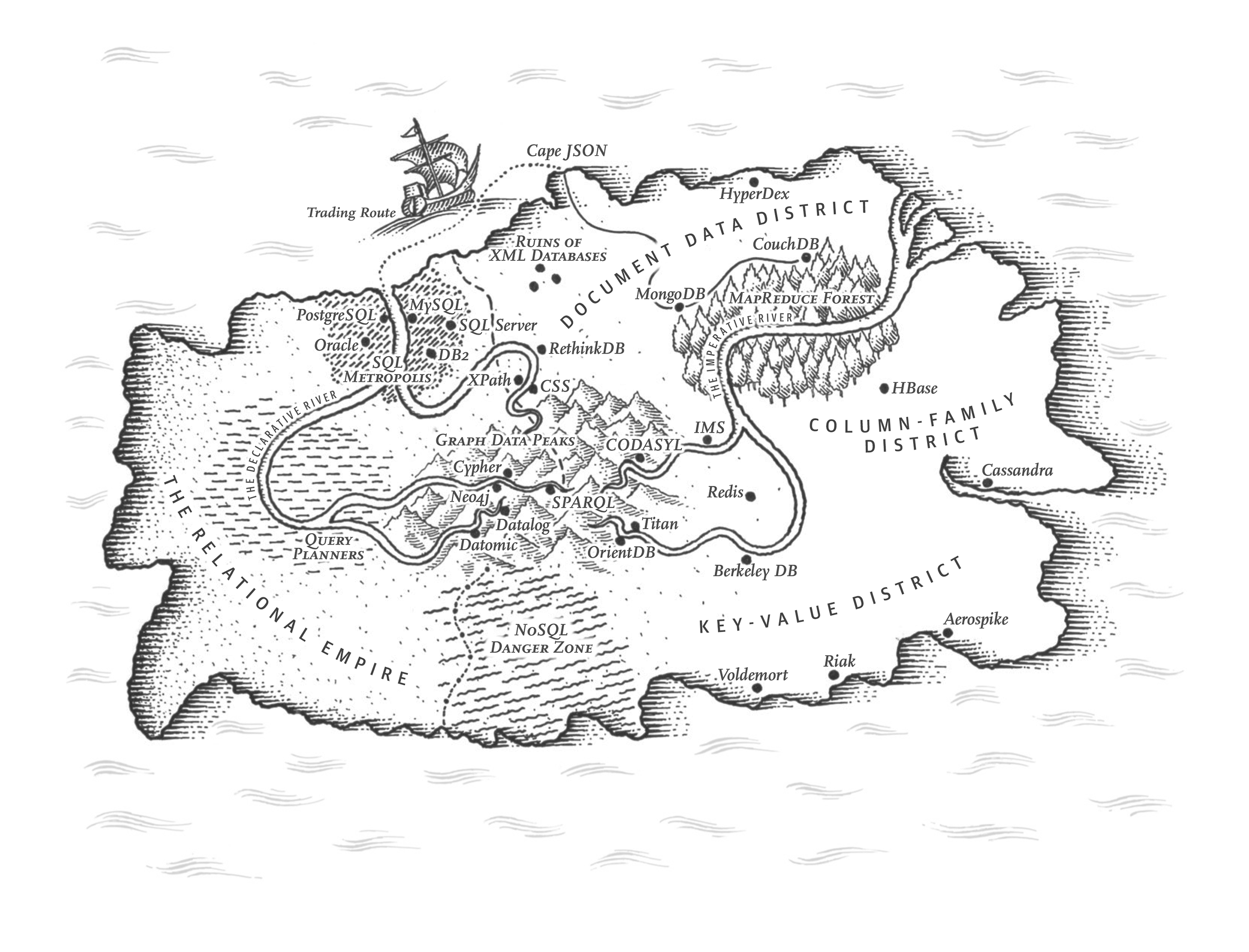
The limits of my language mean the limits of my world.

Ludwig Wittgenstein, Tractatus Logico-Philosophicus (1922)

Data models are perhaps the most important part of developing software, because they have such a profound effect: not only on how the software is written, but also on how we think about the problem that we are solving.

Most applications are built by layering one data model on top of another. For each layer, the key question is: how is it represented in terms of the next-lower layer? For example:

As an application developer, you look at the real world (in which there are people, organizations, goods, actions, money flows, sensors, etc.) and model it in terms of objects or data structures, and APIs that manipulate those data structures. Those structures are often specific to your application.
When you want to store those data structures, you express them in terms of a general-purpose data model, such as JSON or XML documents, tables in a relational database, or vertices and edges in a graph. Those data models are the topic of this chapter.
The engineers who built your database software decided on a way of representing that document/relational/graph data in terms of bytes in memory, on disk, or on a network. The representation may allow the data to be queried, searched, manipulated, and processed in various ways. We will discuss these storage engine designs in Chapter 4.
On yet lower levels, hardware engineers have figured out how to represent bytes in terms of electrical currents, pulses of light, magnetic fields, and more.

In a complex application there may be more intermediary levels, such as APIs built upon APIs, but the basic idea is still the same: each layer hides the complexity of the layers below it by providing a clean data model. These abstractions allow different groups of people—for example, the engineers at the database vendor and the application developers using their database—to work together effectively.

Several different data models are widely used in practice, often for different purposes. Some types of data and some queries are easy to express in one model, and awkward in another. In this chapter we will explore those trade-offs by comparing the relational model, the document model, graph-based data models, event sourcing, and dataframes. We will also briefly look at query languages that allow you to work with these models. This comparison will help you decide when to use which model.

TERMINOLOGY: DECLARATIVE QUERY LANGUAGES

Many of the query languages in this chapter (such as SQL, Cypher, SPARQL, or Datalog) are declarative, which means that you specify the pattern of the data you want—what conditions the results must meet, and how you want the data to be transformed (e.g., sorted, grouped, and aggregated)—but not how to achieve that goal. The database system’s query optimizer can decide which indexes and which join algorithms to use, and in which order to execute various parts of the query.

In contrast, with most programming languages you would have to write an algorithm—i.e., telling the computer which operations to perform in which order. A declarative query language is attractive because it is typically more concise and easier to write than an explicit algorithm. But more importantly, it also hides implementation details of the query engine, which makes it possible for the database system to introduce performance improvements without requiring any changes to queries. ¹.

For example, a database might be able to execute a declarative query in parallel across multiple CPU cores and machines, without you having to worry about how to implement that parallelism ². In a hand-coded algorithm it would be a lot of work to implement such parallel execution yourself.

Relational Model versus Document Model

The best-known data model today is probably that of SQL, based on the relational model proposed by Edgar Codd in 1970 ³: data is organized into relations (called tables in SQL), where each relation is an unordered collection of tuples (rows in SQL).

The relational model was originally a theoretical proposal, and many people at the time doubted whether it could be implemented efficiently. However, by the mid-1980s, relational database management systems (RDBMS) and SQL had become the tools of choice for most people who needed to store and query data with some kind of regular structure. Many data management use cases are still dominated by relational data decades later—for example, business analytics (see “Stars and Snowflakes: Schemas for Analytics”).

Over the years, there have been many competing approaches to data storage and querying. In the 1970s and early 1980s, the network model and the hierarchical model were the main alternatives, but the relational model came to dominate them. Object databases came and went again in the late 1980s and early 1990s. XML databases appeared in the early 2000s, but have only seen niche adoption. Each competitor to the relational model generated a lot of hype in its time, but it never lasted ⁴. Instead, SQL has grown to incorporate other data types besides its relational core—for example, adding support for XML, JSON, and graph data ⁵.

In the 2010s, NoSQL was the latest buzzword that tried to overthrow the dominance of relational databases. NoSQL refers not to a single technology, but a loose set of ideas around new data models, schema flexibility, scalability, and a move towards open source licensing models. Some databases branded themselves as NewSQL, as they aim to provide the scalability of NoSQL systems along with the data model and transactional guarantees of traditional relational databases. The NoSQL and NewSQL ideas have been very influential in the design of data systems, but as the principles have become widely adopted, use of those terms has faded.

One lasting effect of the NoSQL movement is the popularity of the document model, which usually represents data as JSON. This model was originally popularized by specialized document databases such as MongoDB and Couchbase, although most relational databases have now also added JSON support. Compared to relational tables, which are often seen as having a rigid and inflexible schema, JSON documents are thought to be more flexible.

The pros and cons of document and relational data have been debated extensively; let’s examine some of the key points of that debate.

The Object-Relational Mismatch

Much application development today is done in object-oriented programming languages, which leads to a common criticism of the SQL data model: if data is stored in relational tables, an awkward translation layer is required between the objects in the application code and the database model of tables, rows, and columns. The disconnect between the models is sometimes called an impedance mismatch.

Note

The term impedance mismatch is borrowed from electronics. Every electric circuit has a certain impedance (resistance to alternating current) on its inputs and outputs. When you connect one circuit’s output to another one’s input, the power transfer across the connection is maximized if the output and input impedances of the two circuits match. An impedance mismatch can lead to signal reflections and other troubles.

Object-relational mapping (ORM)

Object-relational mapping (ORM) frameworks like ActiveRecord and Hibernate reduce the amount of boilerplate code required for this translation layer, but they are often criticized ⁶. Some commonly cited problems are:

ORMs are complex and can’t completely hide the differences between the two models, so developers still end up having to think about both the relational and the object representations of the data.
ORMs are generally only used for OLTP app development (see “Characterizing Transaction Processing and Analytics”); data engineers making the data available for analytics purposes still need to work with the underlying relational representation, so the design of the relational schema still matters when using an ORM.
Many ORMs work only with relational OLTP databases. Organizations with diverse data systems such as search engines, graph databases, and NoSQL systems might find ORM support lacking.
Some ORMs generate relational schemas automatically, but these might be awkward for the users who are accessing the relational data directly, and they might be inefficient on the underlying database. Customizing the ORM’s schema and query generation can be complex and negate the benefit of using the ORM in the first place.
ORMs make it easy to accidentally write inefficient queries, such as the N+1 query problem ⁷. For example, say you want to display a list of user comments on a page, so you perform one query that returns N comments, each containing the ID of its author. To show the name of the comment author you need to look up the ID in the users table. In hand-written SQL you would probably perform this join in the query and return the author name along with each comment, but with an ORM you might end up making a separate query on the users table for each of the N comments to look up its author, resulting in N+1 database queries in total, which is slower than performing the join in the database. To avoid this problem, you may need to tell the ORM to fetch the author information at the same time as fetching the comments.

Nevertheless, ORMs also have advantages:

For data that is well suited to a relational model, some kind of translation between the persistent relational and the in-memory object representation is inevitable, and ORMs reduce the amount of boilerplate code required for this translation. Complicated queries may still need to be handled outside of the ORM, but the ORM can help with the simple and repetitive cases.
Some ORMs help with caching the results of database queries, which can help reduce the load on the database.
ORMs can also help with managing schema migrations and other administrative activities.

The document data model for one-to-many relationships

Not all data lends itself well to a relational representation; let’s look at an example to explore a limitation of the relational model. Figure 3-1 illustrates how a résumé (a LinkedIn profile) could be expressed in a relational schema. The profile as a whole can be identified by a unique identifier, user_id. Fields like first_name and last_name appear exactly once per user, so they can be modeled as columns on the users table.

Most people have had more than one job in their career (positions), and people may have varying numbers of periods of education and any number of pieces of contact information. One way of representing such one-to-many relationships is to put positions, education, and contact information in separate tables, with a foreign key reference to the users table, as in Figure 3-1.

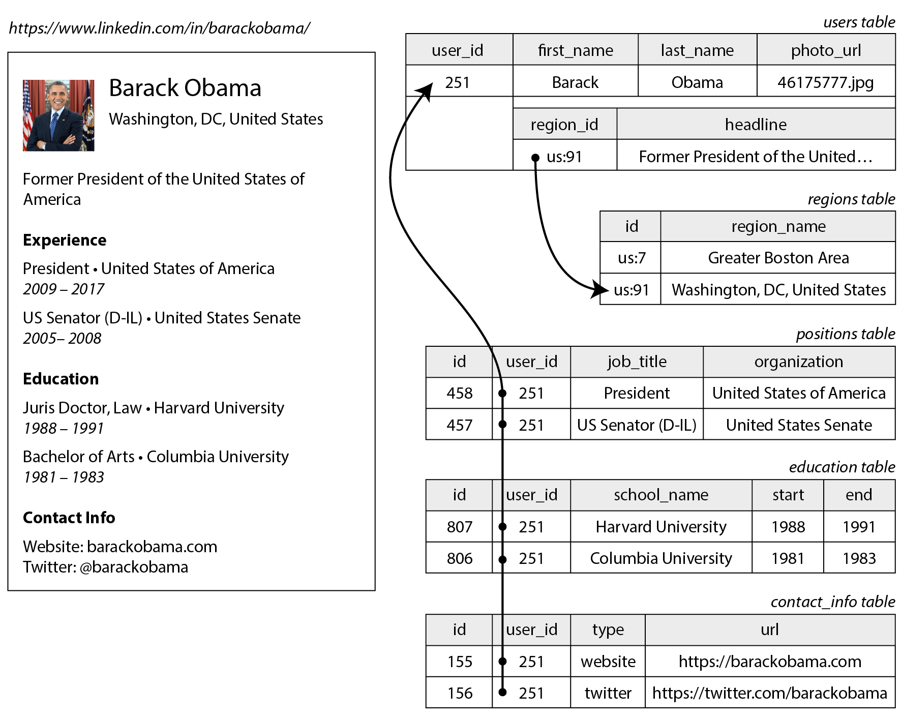
Figure 3-1 Representing a LinkedIn profile using a relational schema.

Another way of representing the same information, which is perhaps more natural and maps more closely to an object structure in application code, is as a JSON document as shown in Example 3-1.

Example 3-1. Representing a LinkedIn profile as a JSON document

{
    "user_id": 251,
    "first_name": "Barack",
    "last_name": "Obama",
    "headline": "Former President of the United States of America",
    "region_id": "us:91",
    "photo_url": "/p/7/000/253/05b/308dd6e.jpg",
    "positions": [
        {"job_title": "President", "organization": "United States of America"},
        {"job_title": "US Senator (D-IL)", "organization": "United States Senate"}
    ],
    "education": [
        {"school_name": "Harvard University", "start": 1988, "end": 1991},
        {"school_name": "Columbia University", "start": 1981, "end": 1983}
    ],
    "contact_info": {
        "website": "https://barackobama.com",
        "twitter": "https://twitter.com/barackobama"
    }
}

Some developers feel that the JSON model reduces the impedance mismatch between the application code and the storage layer. However, as we shall see in Chapter 5, there are also problems with JSON as a data encoding format. The lack of a schema is often cited as an advantage; we will discuss this in “Schema flexibility in the document model”.

The JSON representation has better locality than the multi-table schema in Figure 3-1 (see “Data locality for reads and writes”). If you want to fetch a profile in the relational example, you need to either perform multiple queries (query each table by user_id) or perform a messy multi-way join between the users table and its subordinate tables ⁸. In the JSON representation, all the relevant information is in one place, making the query both faster and simpler.

The one-to-many relationships from the user profile to the user’s positions, educational history, and contact information imply a tree structure in the data, and the JSON representation makes this tree structure explicit (see Figure 3-2).

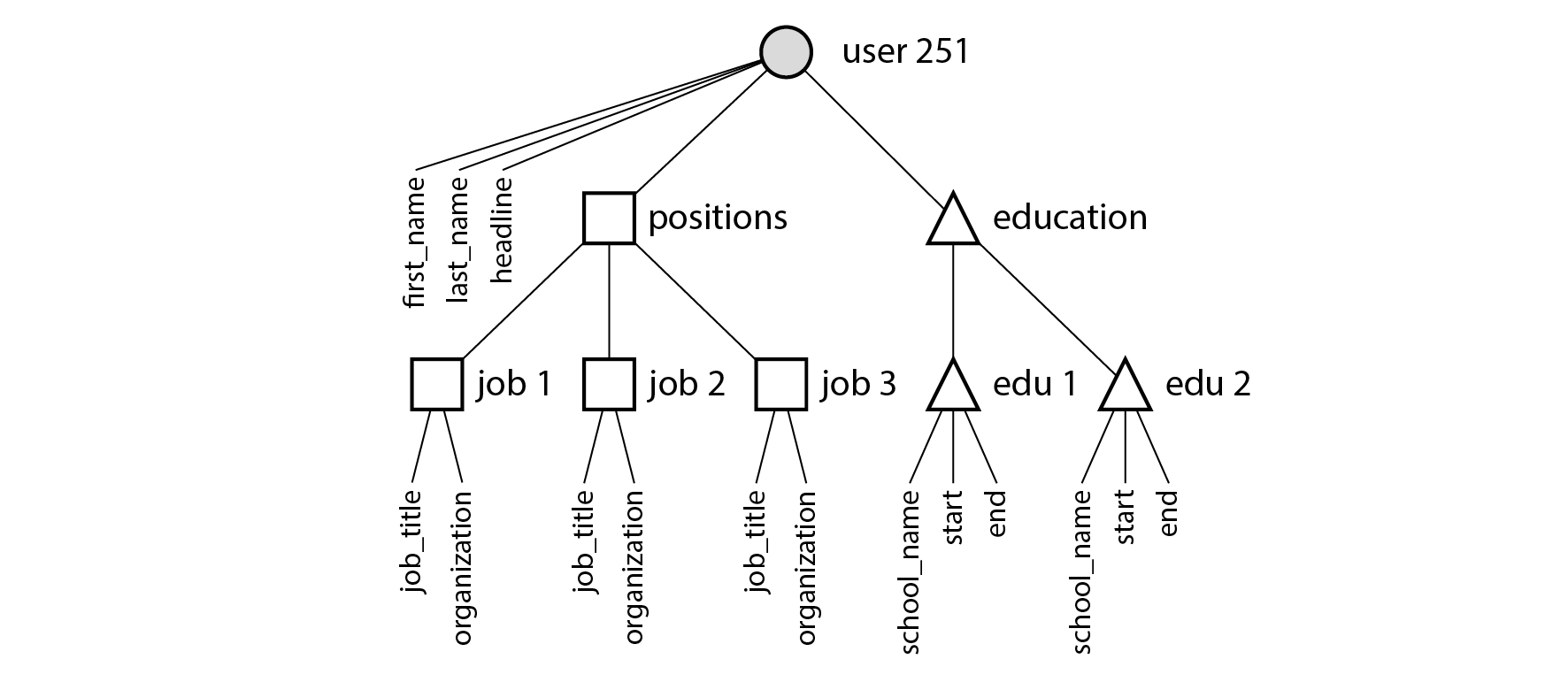
Figure 3-2 One-to-many relationships forming a tree structure.

Note

This type of relationship is sometimes called one-to-few rather than one-to-many, since a résumé typically has a small number of positions ⁹ ¹⁰. In situations where there may be a genuinely large number of related items—say, comments on a celebrity’s social media post, of which there could be many thousands—embedding them all in the same document may be too unwieldy, so the relational approach in Figure 3-1 is preferable.

Normalization, Denormalization, and Joins

In Example 3-1 in the preceding section, region_id is given as an ID, not as the plain-text string "Washington, DC, United States". Why?

If the user interface has a free-text field for entering the region, it makes sense to store it as a plain-text string. But there are advantages to having standardized lists of geographic regions, and letting users choose from a drop-down list or autocompleter:

Consistent style and spelling across profiles
Avoiding ambiguity if there are several places with the same name (if the string were just “Washington”, would it refer to DC or to the state?)
Ease of updating—the name is stored in only one place, so it is easy to update across the board if it ever needs to be changed (e.g., change of a city name due to political events)
Localization support—when the site is translated into other languages, the standardized lists can be localized, so the region can be displayed in the viewer’s language
Better search—e.g., a search for people on the US East Coast can match this profile, because the list of regions can encode the fact that Washington is located on the East Coast (which is not apparent from the string "Washington, DC")

Whether you store an ID or a text string is a question of normalization. When you use an ID, your data is more normalized: the information that is meaningful to humans (such as the text Washington, DC) is stored in only one place, and everything that refers to it uses an ID (which only has meaning within the database). When you store the text directly, you are duplicating the human-meaningful information in every record that uses it; this representation is denormalized.

The advantage of using an ID is that because it has no meaning to humans, it never needs to change: the ID can remain the same, even if the information it identifies changes. Anything that is meaningful to humans may need to change sometime in the future—and if that information is duplicated, all the redundant copies need to be updated. That requires more code, more write operations, more disk space, and risks inconsistencies (where some copies of the information are updated but others aren’t).

The downside of a normalized representation is that every time you want to display a record containing an ID, you have to do an additional lookup to resolve the ID into something human-readable. In a relational data model, this is done using a join, for example:

SELECT users.*, regions.region_name
    FROM users
    JOIN regions ON users.region_id = regions.id
    WHERE users.id = 251;

Document databases can store both normalized and denormalized data, but they are often associated with denormalization—partly because the JSON data model makes it easy to store additional, denormalized fields, and partly because the weak support for joins in many document databases makes normalization inconvenient. Some document databases don’t support joins at all, so you have to perform them in application code—that is, you first fetch a document containing an ID, and then perform a second query to resolve that ID into another document. In MongoDB, it is also possible to perform a join using the $lookup operator in an aggregation pipeline:

db.users.aggregate([
    { $match: { _id: 251 } },
    { $lookup: {
        from: "regions",
        localField: "region_id",
        foreignField: "_id",
        as: "region"
    } }
])

Trade-offs of normalization

In the résumé example, while the region_id field is a reference into a standardized set of regions, the name of the organization (the company or government where the person worked) and school_name (where they studied) are just strings. This representation is denormalized: many people may have worked at the same company, but there is no ID linking them.

Perhaps the organization and school should be entities instead, and the profile should reference their IDs instead of their names? The same arguments for referencing the ID of a region also apply here. For example, say we wanted to include the logo of the school or company in addition to their name:

In a denormalized representation, we would include the image URL of the logo on every individual person’s profile; this makes the JSON document self-contained, but it creates a headache if we ever need to change the logo, because we now need to find all of the occurrences of the old URL and update them ⁹.
In a normalized representation, we would create an entity representing an organization or school, and store its name, logo URL, and perhaps other attributes (description, news feed, etc.) once on that entity. Every résumé that mentions the organization would then simply reference its ID, and updating the logo is easy.

As a general principle, normalized data is usually faster to write (since there is only one copy), but slower to query (since it requires joins); denormalized data is usually faster to read (fewer joins), but more expensive to write (more copies to update, more disk space used). You might find it helpful to view denormalization as a form of derived data (“Systems of Record and Derived Data”), since you need to set up a process for updating the redundant copies of the data.

Besides the cost of performing all these updates, you also need to consider the consistency of the database if a process crashes halfway through making its updates. Databases that offer atomic transactions (see “Atomicity”) make it easier to remain consistent, but not all databases offer atomicity across multiple documents. It is also possible to ensure consistency through stream processing, which we discuss in “Keeping Systems in Sync”.

Normalization tends to be better for OLTP systems, where both reads and updates need to be fast; analytics systems often fare better with denormalized data, since they perform updates in bulk, and the performance of read-only queries is the dominant concern. Moreover, in systems of small to moderate scale, a normalized data model is often best, because you don’t have to worry about keeping multiple copies of the data consistent with each other, and the cost of performing joins is acceptable. However, in very large-scale systems, the cost of joins can become problematic.

In “Case Study: Social Network Home Timelines” we compared a normalized representation (Figure 2-1) and a denormalized one (precomputed, materialized timelines): here, the join between posts and follows was too expensive, and the materialized timeline is a cache of the result of that join. The fan-out process that inserts a new post into followers’ timelines was our way of keeping the denormalized representation consistent.

However, the implementation of materialized timelines at X (formerly Twitter) does not store the actual text of each post: each entry actually only stores the post ID, the ID of the user who posted it, and a little bit of extra information to identify reposts and replies ¹¹. In other words, it is a precomputed result of (approximately) the following query:

SELECT posts.id, posts.sender_id 
    FROM posts
    JOIN follows ON posts.sender_id = follows.followee_id
    WHERE follows.follower_id = current_user
    ORDER BY posts.timestamp DESC
    LIMIT 1000

This means that whenever the timeline is read, the service still needs to perform two joins: look up the post ID to fetch the actual post content (as well as statistics such as the number of likes and replies), and look up the sender’s profile by ID (to get their username, profile picture, and other details). This process of looking up the human-readable information by ID is called hydrating the IDs, and it is essentially a join performed in application code ¹¹.

The reason for storing only IDs in the precomputed timeline is that the data they refer to is fast-changing: the number of likes and replies may change multiple times per second on a popular post, and some users regularly change their username or profile photo. Since the timeline should show the latest like count and profile picture when it is viewed, it would not make sense to denormalize this information into the materialized timeline. Moreover, the storage cost would be increased significantly by such denormalization.

This example shows that having to perform joins when reading data is not, as sometimes claimed, an impediment to creating high-performance, scalable services. Hydrating post ID and user ID is actually a fairly easy operation to scale, since it parallelizes well, and the cost doesn’t depend on the number of accounts you are following or the number of followers you have.

If you need to decide whether to denormalize something in your application, the social network case study shows that the choice is not immediately obvious: the most scalable approach may involve denormalizing some things and leaving other things normalized. You will have to carefully consider how often the information changes, and the cost of reads and writes (which might be dominated by outliers, such as users with many follows/followers in the case of a typical social network). Normalization and denormalization are not inherently good or bad—they are just a trade-off in terms of performance of reads and writes, as well as the amount of effort to implement.

Many-to-One and Many-to-Many Relationships

While positions and education in Figure 3-1 are examples of one-to-many or one-to-few relationships (one résumé has several positions, but each position belongs only to one résumé), the region_id field is an example of a many-to-one relationship (many people live in the same region, but we assume that each person lives in only one region at any one time).

If we introduce entities for organizations and schools, and reference them by ID from the résumé, then we also have many-to-many relationships (one person has worked for several organizations, and an organization has several past or present employees). In a relational model, such a relationship is usually represented as an associative table or join table, as shown in Figure 3-3: each position associates one user ID with one organization ID.

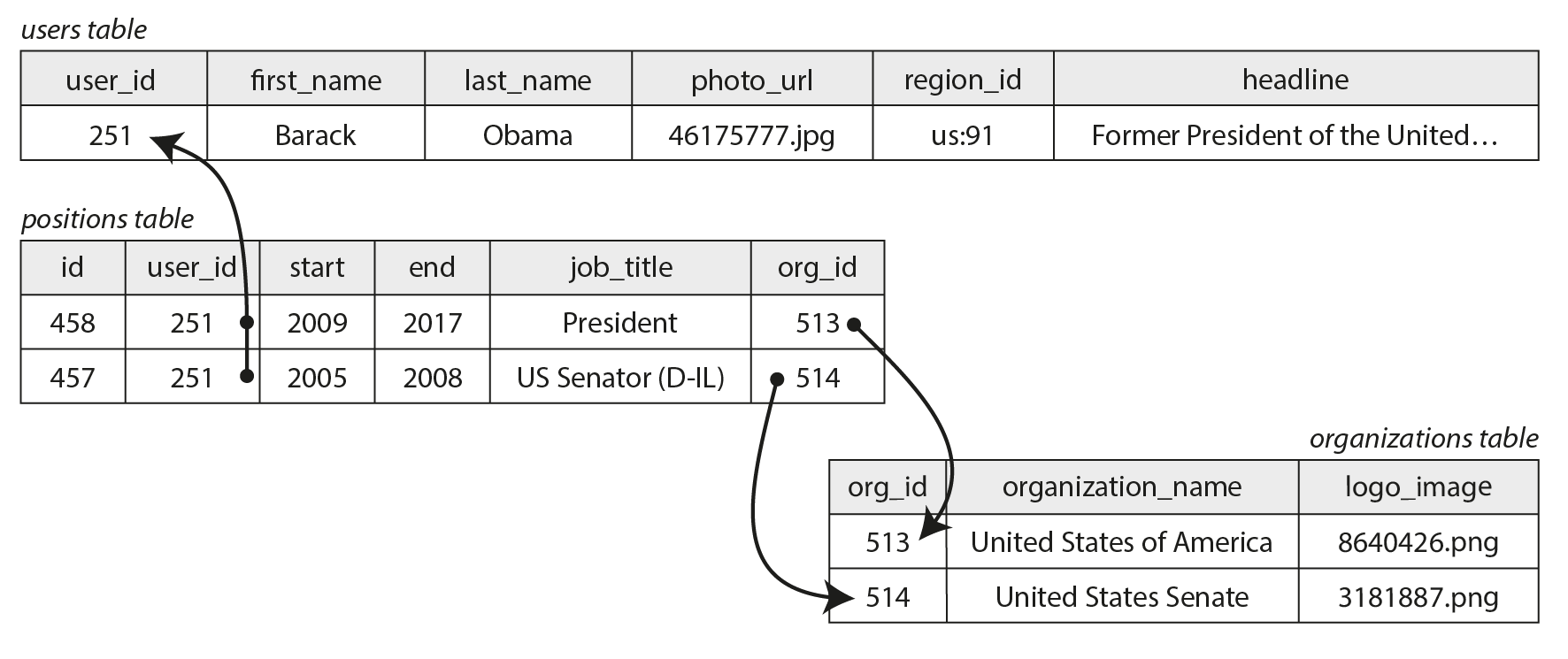
Figure 3-3 Many-to-many relationships in the relational model.

Many-to-one and many-to-many relationships do not easily fit within one self-contained JSON document; they lend themselves more to a normalized representation. In a document model, one possible representation is given in Example 3-2 and illustrated in Figure 3-4: the data within each dotted rectangle can be grouped into one document, but the links to organizations and schools are best represented as references to other documents.

Example 3-2. A résumé that references organizations by ID.

{
    "user_id": 251,
    "first_name": "Barack",
    "last_name": "Obama",
    "positions": [
        {"start": 2009, "end": 2017, "job_title": "President", "org_id": 513},
        {"start": 2005, "end": 2008, "job_title": "US Senator (D-IL)", "org_id": 514}
    ],
    ...
}

Figure 3-4 Many-to-many relationships in the document model: the data within each dotted box can be grouped into one document.

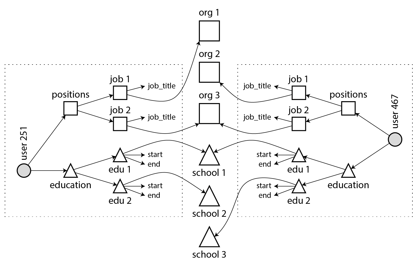
Many-to-many relationships often need to be queried in “both directions”: for example, finding all of the organizations that a particular person has worked for, and finding all of the people who have worked at a particular organization. One way of enabling such queries is to store ID references on both sides, i.e., a résumé includes the ID of each organization where the person has worked, and the organization document includes the IDs of the résumés that mention that organization. This representation is denormalized, since the relationship is stored in two places, which could become inconsistent with each other.

A normalized representation stores the relationship in only one place, and relies on secondary indexes (which we discuss in Chapter 4) to allow the relationship to be efficiently queried in both directions. In the relational schema of Figure 3-3, we would tell the database to create indexes on both the user_id and the org_id columns of the positions table.

In the document model of Example 3-2, the database needs to index the org_id field of objects inside the positions array. Many document databases and relational databases with JSON support are able to create such indexes on values inside a document.

Stars and Snowflakes: Schemas for Analytics

Data warehouses (see “Data Warehousing”) are usually relational, and there are a few widely-used conventions for the structure of tables in a data warehouse: a star schema, snowflake schema, dimensional modeling ¹², and one big table (OBT). These structures are optimized for the needs of business analysts. ETL processes translate data from operational systems into this schema.

Figure 3-5 shows an example of a star schema that might be found in the data warehouse of a grocery retailer. At the center of the schema is a so-called fact table (in this example, it is called fact_sales). Each row of the fact table represents an event that occurred at a particular time (here, each row represents a customer’s purchase of a product). If we were analyzing website traffic rather than retail sales, each row might represent a page view or a click by a user.

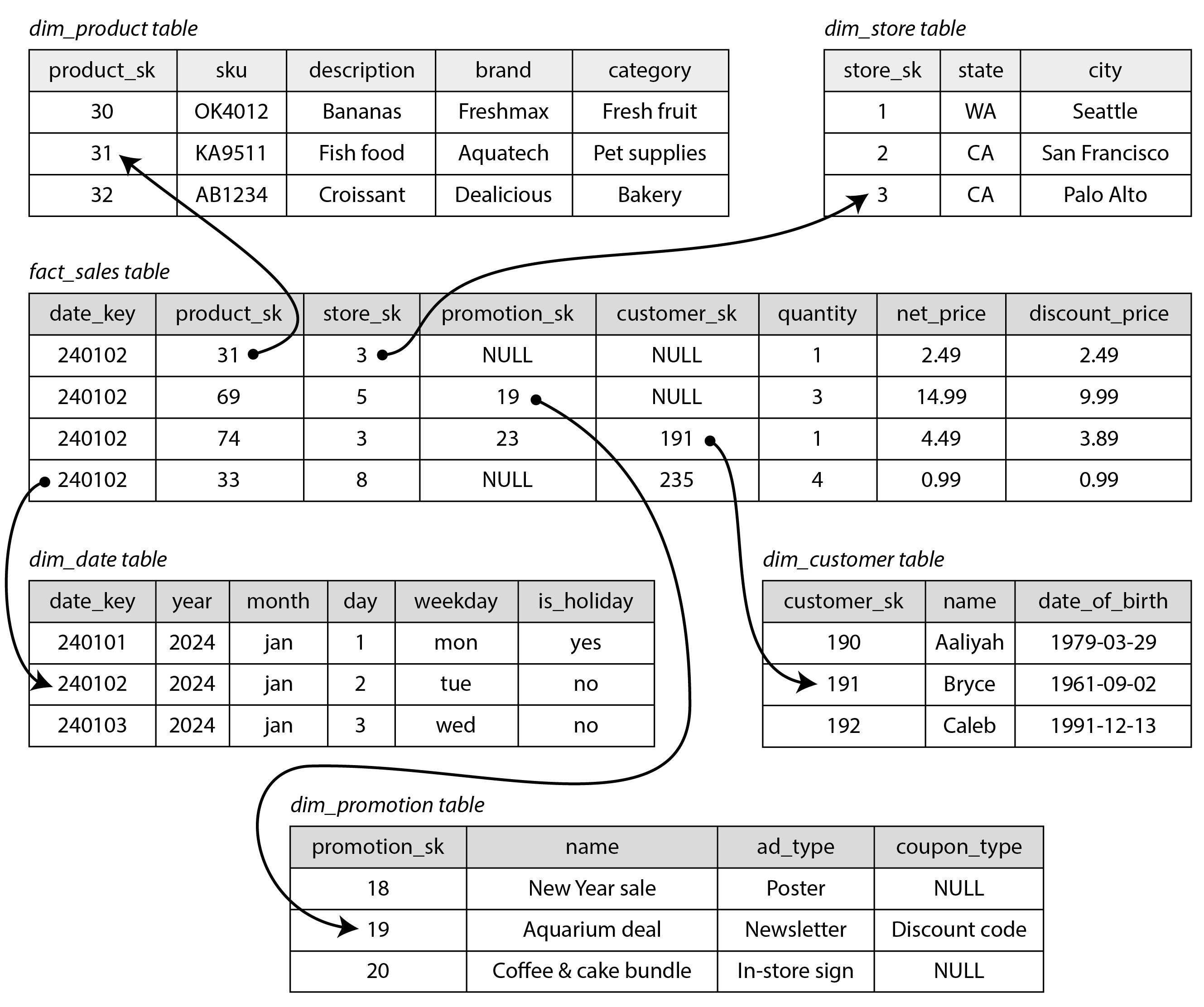
Figure 3-5 Example of a star schema for use in a data warehouse.

Usually, facts are captured as individual events, because this allows maximum flexibility of analysis later. However, this means that the fact table can become extremely large. A big enterprise may have many petabytes of transaction history in its data warehouse, mostly represented as fact tables.

Some of the columns in the fact table are attributes, such as the price at which the product was sold and the cost of buying it from the supplier (allowing the profit margin to be calculated). Other columns in the fact table are foreign key references to other tables, called dimension tables. As each row in the fact table represents an event, the dimensions represent the who, what, where, when, how, and why of the event.

For example, in Figure 3-5, one of the dimensions is the product that was sold. Each row in the dim_product table represents one type of product that is for sale, including its stock-keeping unit (SKU), description, brand name, category, fat content, package size, etc. Each row in the fact_sales table uses a foreign key to indicate which product was sold in that particular transaction. Queries often involve multiple joins to multiple dimension tables.

Even date and time are often represented using dimension tables, because this allows additional information about dates (such as public holidays) to be encoded, allowing queries to differentiate between sales on holidays and non-holidays.

Figure 3-5 is an example of a star schema. The name comes from the fact that when the table relationships are visualized, the fact table is in the middle, surrounded by its dimension tables; the connections to these tables are like the rays of a star.

A variation of this template is known as the snowflake schema, where dimensions are further broken down into subdimensions. For example, there could be separate tables for brands and product categories, and each row in the dim_product table could reference the brand and category as foreign keys, rather than storing them as strings in the dim_product table. Snowflake schemas are more normalized than star schemas, but star schemas are often preferred because they are simpler for analysts to work with ¹².

In a typical data warehouse, tables are often quite wide: fact tables often have over 100 columns, sometimes several hundred. Dimension tables can also be wide, as they include all the metadata that may be relevant for analysis—for example, the dim_store table may include details of which services are offered at each store, whether it has an in-store bakery, the square footage, the date when the store was first opened, when it was last remodeled, how far it is from the nearest highway, etc.

A star or snowflake schema consists mostly of many-to-one relationships (e.g., many sales occur for one particular product, in one particular store), represented as the fact table having foreign keys into dimension tables, or dimensions into sub-dimensions. In principle, other types of relationship could exist, but they are often denormalized in order to simplify queries. For example, if a customer buys several different products at once, that multi-item transaction is not represented explicitly; instead, there is a separate row in the fact table for each product purchased, and those facts all just happen to have the same customer ID, store ID, and timestamp.

Some data warehouse schemas take denormalization even further and leave out the dimension tables entirely, folding the information in the dimensions into denormalized columns on the fact table instead (essentially, precomputing the join between the fact table and the dimension tables). This approach is known as one big table (OBT), and while it requires more storage space, it sometimes enables faster queries ¹³.

In the context of analytics, such denormalization is unproblematic, since the data typically represents a log of historical data that is not going to change (except maybe for occasionally correcting an error). The issues of data consistency and write overheads that occur with denormalization in OLTP systems are not as pressing in analytics.

When to Use Which Model

The main arguments in favor of the document data model are schema flexibility, better performance due to locality, and that for some applications it is closer to the object model used by the application. The relational model counters by providing better support for joins, many-to-one, and many-to-many relationships. Let’s examine these arguments in more detail.

If the data in your application has a document-like structure (i.e., a tree of one-to-many relationships, where typically the entire tree is loaded at once), then it’s probably a good idea to use a document model. The relational technique of shredding—splitting a document-like structure into multiple tables (like positions, education, and contact_info in Figure 3-1) — can lead to cumbersome schemas and unnecessarily complicated application code.

The document model has limitations: for example, you cannot refer directly to a nested item within a document, but instead you need to say something like “the second item in the list of positions for user 251”. If you do need to reference nested items, a relational approach works better, since you can refer to any item directly by its ID.

Some applications allow the user to choose the order of items: for example, imagine a to-do list or issue tracker where the user can drag and drop tasks to reorder them. The document model supports such applications well, because the items (or their IDs) can simply be stored in a JSON array to determine their order. In relational databases there isn’t a standard way of representing such reorderable lists, and various tricks are used: sorting by an integer column (requiring renumbering when you insert into the middle), a linked list of IDs, or fractional indexing ¹⁴ ¹⁵ ¹⁶.

Schema flexibility in the document model

Most document databases, and the JSON support in relational databases, do not enforce any schema on the data in documents. XML support in relational databases usually comes with optional schema validation. No schema means that arbitrary keys and values can be added to a document, and when reading, clients have no guarantees as to what fields the documents may contain.

Document databases are sometimes called schemaless, but that’s misleading, as the code that reads the data usually assumes some kind of structure—i.e., there is an implicit schema, but it is not enforced by the database ¹⁷. A more accurate term is schema-on-read (the structure of the data is implicit, and only interpreted when the data is read), in contrast with schema-on-write (the traditional approach of relational databases, where the schema is explicit and the database ensures all data conforms to it when the data is written) ¹⁸.

Schema-on-read is similar to dynamic (runtime) type checking in programming languages, whereas schema-on-write is similar to static (compile-time) type checking. Just as the advocates of static and dynamic type checking have big debates about their relative merits ¹⁹, enforcement of schemas in database is a contentious topic, and in general there’s no right or wrong answer.

The difference between the approaches is particularly noticeable in situations where an application wants to change the format of its data. For example, say you are currently storing each user’s full name in one field, and you instead want to store the first name and last name separately ²⁰. In a document database, you would just start writing new documents with the new fields and have code in the application that handles the case when old documents are read. For example:

if (user && user.name && !user.first_name) {
    // Documents written before Dec 8, 2023 don't have first_name
    user.first_name = user.name.split(" ")[0];
}

The downside of this approach is that every part of your application that reads from the database now needs to deal with documents in old formats that may have been written a long time in the past. On the other hand, in a schema-on-write database, you would typically perform a migration along the lines of:

ALTER TABLE users ADD COLUMN first_name text DEFAULT NULL;
UPDATE users SET first_name = split_part(name, ' ', 1); -- PostgreSQL
UPDATE users SET first_name = substring_index(name, ' ', 1); -- MySQL

In most relational databases, adding a column with a default value is fast and unproblematic, even on large tables. However, running the UPDATE statement is likely to be slow on a large table, since every row needs to be rewritten, and other schema operations (such as changing the data type of a column) also typically require the entire table to be copied.

Various tools exist to allow this type of schema changes to be performed in the background without downtime ²¹ ²² ²³ ²⁴, but performing such migrations on large databases remains operationally challenging. Complicated migrations can be avoided by only adding the first_name column with a default value of NULL (which is fast), and filling it in at read time, like you would with a document database.

The schema-on-read approach is advantageous if the items in the collection don’t all have the same structure for some reason (i.e., the data is heterogeneous)—for example, because:

There are many different types of objects, and it is not practicable to put each type of object in its own table.
The structure of the data is determined by external systems over which you have no control and which may change at any time.

In situations like these, a schema may hurt more than it helps, and schemaless documents can be a much more natural data model. But in cases where all records are expected to have the same structure, schemas are a useful mechanism for documenting and enforcing that structure. We will discuss schemas and schema evolution in more detail in Chapter 5.

Data locality for reads and writes

A document is usually stored as a single continuous string, encoded as JSON, XML, or a binary variant thereof (such as MongoDB’s BSON). If your application often needs to access the entire document (for example, to render it on a web page), there is a performance advantage to this storage locality. If data is split across multiple tables, like in Figure 3-1, multiple index lookups are required to retrieve it all, which may require more disk seeks and take more time.

The locality advantage only applies if you need large parts of the document at the same time. The database typically needs to load the entire document, which can be wasteful if you only need to access a small part of a large document. On updates to a document, the entire document usually needs to be rewritten. For these reasons, it is generally recommended that you keep documents fairly small and avoid frequent small updates to a document.

However, the idea of storing related data together for locality is not limited to the document model. For example, Google’s Spanner database offers the same locality properties in a relational data model, by allowing the schema to declare that a table’s rows should be interleaved (nested) within a parent table ²⁵. Oracle allows the same, using a feature called multi-table index cluster tables ²⁶. The wide-column data model popularized by Google’s Bigtable, and used e.g. in HBase and Accumulo, has a concept of column families, which have a similar purpose of managing locality ²⁷.

Query languages for documents

Another difference between a relational and a document database is the language or API that you use to query it. Most relational databases are queried using SQL, but document databases are more varied. Some allow only key-value access by primary key, while others also offer secondary indexes to query for values inside documents, and some provide rich query languages.

XML databases are often queried using XQuery and XPath, which are designed to allow complex queries, including joins across multiple documents, and also format their results as XML ²⁸. JSON Pointer ²⁹ and JSONPath ³⁰ provide an equivalent to XPath for JSON.

MongoDB’s aggregation pipeline, whose $lookup operator for joins we saw in “Normalization, Denormalization, and Joins”, is an example of a query language for collections of JSON documents.

Let’s look at another example to get a feel for this language—this time an aggregation, which is especially needed for analytics. Imagine you are a marine biologist, and you add an observation record to your database every time you see animals in the ocean. Now you want to generate a report saying how many sharks you have sighted per month. In PostgreSQL you might express that query like this:

SELECT date_trunc('month', observation_timestamp) AS observation_month, ❶ 
    sum(num_animals) AS total_animals
FROM observations
WHERE family = 'Sharks'
GROUP BY observation_month;

❶ : The date_trunc('month', timestamp) function determines the calendar month containing timestamp, and returns another timestamp representing the beginning of that month. In other words, it rounds a timestamp down to the nearest month.

This query first filters the observations to only show species in the Sharks family, then groups the observations by the calendar month in which they occurred, and finally adds up the number of animals seen in all observations in that month. The same query can be expressed using MongoDB’s aggregation pipeline as follows:

db.observations.aggregate([
    { $match: { family: "Sharks" } },
    { $group: {
    _id: {
        year: { $year: "$observationTimestamp" },
        month: { $month: "$observationTimestamp" }
    },
    totalAnimals: { $sum: "$numAnimals" }
    } }
]);

The aggregation pipeline language is similar in expressiveness to a subset of SQL, but it uses a JSON-based syntax rather than SQL’s English-sentence-style syntax; the difference is perhaps a matter of taste.

Convergence of document and relational databases

Document databases and relational databases started out as very different approaches to data management, but they have grown more similar over time ³¹. Relational databases added support for JSON types and query operators, and the ability to index properties inside documents. Some document databases (such as MongoDB, Couchbase, and RethinkDB) added support for joins, secondary indexes, and declarative query languages.

This convergence of the models is good news for application developers, because the relational model and the document model work best when you can combine both in the same database. Many document databases need relational-style references to other documents, and many relational databases have sections where schema flexibility is beneficial. Relational-document hybrids are a powerful combination.

Note

Codd’s original description of the relational model ³ actually allowed something similar to JSON within a relational schema. He called it nonsimple domains. The idea was that a value in a row doesn’t have to just be a primitive datatype like a number or a string, but it could also be a nested relation (table)—so you can have an arbitrarily nested tree structure as a value, much like the JSON or XML support that was added to SQL over 30 years later.

Graph-Like Data Models

We saw earlier that the type of relationships is an important distinguishing feature between different data models. If your application has mostly one-to-many relationships (tree-structured data) and few other relationships between records, the document model is appropriate.

But what if many-to-many relationships are very common in your data? The relational model can handle simple cases of many-to-many relationships, but as the connections within your data become more complex, it becomes more natural to start modeling your data as a graph.

A graph consists of two kinds of objects: vertices (also known as nodes or entities) and edges (also known as relationships or arcs). Many kinds of data can be modeled as a graph. Typical examples include:

Social graphs: Vertices are people, and edges indicate which people know each other.
The web graph: Vertices are web pages, and edges indicate HTML links to other pages.
Road or rail networks: Vertices are junctions, and edges represent the roads or railway lines between them.

Well-known algorithms can operate on these graphs: for example, map navigation apps search for the shortest path between two points in a road network, and PageRank can be used on the web graph to determine the popularity of a web page and thus its ranking in search results ³².

Graphs can be represented in several different ways. In the adjacency list model, each vertex stores the IDs of its neighbor vertices that are one edge away. Alternatively, you can use an adjacency matrix, a two-dimensional array where each row and each column corresponds to a vertex, where the value is zero when there is no edge between the row vertex and the column vertex, and where the value is one if there is an edge. The adjacency list is good for graph traversals, and the matrix is good for machine learning (see “Dataframes, Matrices, and Arrays”).

In the examples just given, all the vertices in a graph represent the same kind of thing (people, web pages, or road junctions, respectively). However, graphs are not limited to such homogeneous data: an equally powerful use of graphs is to provide a consistent way of storing completely different types of objects in a single database. For example:

Facebook maintains a single graph with many different types of vertices and edges: vertices represent people, locations, events, checkins, and comments made by users; edges indicate which people are friends with each other, which checkin happened in which location, who commented on which post, who attended which event, and so on ³³.
Knowledge graphs are used by search engines to record facts about entities that often occur in search queries, such as organizations, people, and places ³⁴. This information is obtained by crawling and analyzing the text on websites; some websites, such as Wikidata, also publish graph data in a structured form.

There are several different, but related, ways of structuring and querying data in graphs. In this section we will discuss the property graph model (implemented by Neo4j, Memgraph, KùzuDB ³⁵, and others ³⁶) and the triple-store model (implemented by Datomic, AllegroGraph, Blazegraph, and others). These models are fairly similar in what they can express, and some graph databases (such as Amazon Neptune) support both models.

We will also look at four query languages for graphs (Cypher, SPARQL, Datalog, and GraphQL), as well as SQL support for querying graphs. Other graph query languages exist, such as Gremlin ³⁷, but these will give us a representative overview.

To illustrate these different languages and models, this section uses the graph shown in Figure 3-6 as running example. It could be taken from a social network or a genealogical database: it shows two people, Lucy from Idaho and Alain from Saint-Lô, France. They are married and living in London. Each person and each location is represented as a vertex, and the relationships between them as edges. This example will help demonstrate some queries that are easy in graph databases, but difficult in other models.

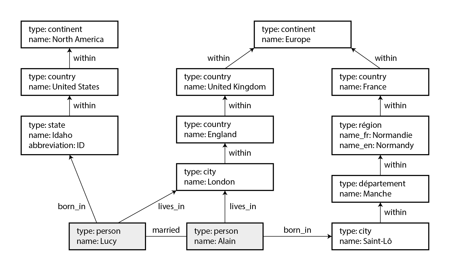
Figure 3-6 Example of graph-structured data (boxes represent vertices, arrows represent edges).

Property Graphs

In the property graph (also known as labeled property graph) model, each vertex consists of:

A unique identifier
A label (string) to describe what type of object this vertex represents
A set of outgoing edges
A set of incoming edges
A collection of properties (key-value pairs)

Each edge consists of:

A unique identifier
The vertex at which the edge starts (the tail vertex)
The vertex at which the edge ends (the head vertex)
A label to describe the kind of relationship between the two vertices
A collection of properties (key-value pairs)

You can think of a graph store as consisting of two relational tables, one for vertices and one for edges, as shown in Example 3-3 (this schema uses the PostgreSQL jsonb datatype to store the properties of each vertex or edge). The head and tail vertex are stored for each edge; if you want the set of incoming or outgoing edges for a vertex, you can query the edges table by head_vertex or tail_vertex, respectively.

Example 3-3. Representing a property graph using a relational schema

CREATE TABLE vertices (
    vertex_id integer PRIMARY KEY,
    label text,
    properties jsonb
);

CREATE TABLE edges (
    edge_id integer PRIMARY KEY,
    tail_vertex integer REFERENCES vertices (vertex_id),
    head_vertex integer REFERENCES vertices (vertex_id),
    label text,
    properties jsonb
);

CREATE INDEX edges_tails ON edges (tail_vertex);
CREATE INDEX edges_heads ON edges (head_vertex);

Some important aspects of this model are:

Any vertex can have an edge connecting it with any other vertex. There is no schema that restricts which kinds of things can or cannot be associated.
Given any vertex, you can efficiently find both its incoming and its outgoing edges, and thus traverse the graph—i.e., follow a path through a chain of vertices—both forward and backward. (That’s why Example 3-3 has indexes on both the tail_vertex and head_vertex columns.)
By using different labels for different kinds of vertices and relationships, you can store several different kinds of information in a single graph, while still maintaining a clean data model.

The edges table is like the many-to-many associative table/join table we saw in “Many-to-One and Many-to-Many Relationships”, generalized to allow many different types of relationship to be stored in the same table. There may also be indexes on the labels and the properties, allowing vertices or edges with certain properties to be found efficiently.

Note

A limitation of graph models is that an edge can only associate two vertices with each other, whereas a relational join table can represent three-way or even higher-degree relationships by having multiple foreign key references on a single row. Such relationships can be represented in a graph by creating an additional vertex corresponding to each row of the join table, and edges to/from that vertex, or by using a hypergraph.

Those features give graphs a great deal of flexibility for data modeling, as illustrated in Figure 3-6. The figure shows a few things that would be difficult to express in a traditional relational schema, such as different kinds of regional structures in different countries (France has départements and régions, whereas the US has counties and states), quirks of history such as a country within a country (ignoring for now the intricacies of sovereign states and nations), and varying granularity of data (Lucy’s current residence is specified as a city, whereas her place of birth is specified only at the level of a state).

You could imagine extending the graph to also include many other facts about Lucy and Alain, or other people. For instance, you could use it to indicate any food allergies they have (by introducing a vertex for each allergen, and an edge between a person and an allergen to indicate an allergy), and link the allergens with a set of vertices that show which foods contain which substances. Then you could write a query to find out what is safe for each person to eat. Graphs are good for evolvability: as you add features to your application, a graph can easily be extended to accommodate changes in your application’s data structures.

The Cypher Query Language

Cypher is a query language for property graphs, originally created for the Neo4j graph database, and later developed into an open standard as openCypher ³⁸. Besides Neo4j, Cypher is supported by Memgraph, KùzuDB ³⁵, Amazon Neptune, Apache AGE (with storage in PostgreSQL), and others. It is named after a character in the movie The Matrix and is not related to ciphers in cryptography ³⁹.

Example 3-4 shows the Cypher query to insert the lefthand portion of Figure 3-6 into a graph database. The rest of the graph can be added similarly. Each vertex is given a symbolic name like usa or idaho. That name is not stored in the database, but only used internally within the query to create edges between the vertices, using an arrow notation: (idaho) -[:WITHIN]-> (usa) creates an edge labeled WITHIN, with idaho as the tail node and usa as the head node.

Example 3-4. A subset of the data in Figure 3-6, represented as a Cypher query

CREATE
    (namerica :Location {name:'North America', type:'continent'}),
    (usa :Location {name:'United States', type:'country' }),
    (idaho :Location {name:'Idaho', type:'state' }),
    (lucy :Person {name:'Lucy' }),
    (idaho) -[:WITHIN ]-> (usa) -[:WITHIN]-> (namerica),
    (lucy) -[:BORN_IN]-> (idaho)

When all the vertices and edges of Figure 3-6 are added to the database, we can start asking interesting questions: for example, find the names of all the people who emigrated from the United States to Europe. That is, find all the vertices that have a BORN_IN edge to a location within the US, and also a LIVES_IN edge to a location within Europe, and return the name property of each of those vertices.

Example 3-5 shows how to express that query in Cypher. The same arrow notation is used in a MATCH clause to find patterns in the graph: (person) -[:BORN_IN]-> () matches any two vertices that are related by an edge labeled BORN_IN. The tail vertex of that edge is bound to the variable person, and the head vertex is left unnamed.

Example 3-5. Cypher query to find people who emigrated from the US to Europe

MATCH
    (person) -[:BORN_IN]-> () -[:WITHIN*0..]-> (:Location {name:'United States'}),
    (person) -[:LIVES_IN]-> () -[:WITHIN*0..]-> (:Location {name:'Europe'})
RETURN person.name

The query can be read as follows:

Find any vertex (call it person) that meets both of the following conditions:

person has an outgoing BORN_IN edge to some vertex. From that vertex, you can follow a chain of outgoing WITHIN edges until eventually you reach a vertex of type Location, whose name property is equal to "United States".

That same person vertex also has an outgoing LIVES_IN edge. Following that edge, and then a chain of outgoing WITHIN edges, you eventually reach a vertex of type Location, whose name property is equal to "Europe".

For each such person vertex, return the name property.

There are several possible ways of executing the query. The description given here suggests that you start by scanning all the people in the database, examine each person’s birthplace and residence, and return only those people who meet the criteria.

But equivalently, you could start with the two Location vertices and work backward. If there is an index on the name property, you can efficiently find the two vertices representing the US and Europe. Then you can proceed to find all locations (states, regions, cities, etc.) in the US and Europe respectively by following all incoming WITHIN edges. Finally, you can look for people who can be found through an incoming BORN_IN or LIVES_IN edge at one of the location vertices.

Graph Queries in SQL

Example 3-3 suggested that graph data can be represented in a relational database. But if we put graph data in a relational structure, can we also query it using SQL?

The answer is yes, but with some difficulty. Every edge that you traverse in a graph query is effectively a join with the edges table. In a relational database, you usually know in advance which joins you need in your query. On the other hand, in a graph query, you may need to traverse a variable number of edges before you find the vertex you’re looking for—that is, the number of joins is not fixed in advance.

In our example, that happens in the () -[:WITHIN*0..]-> () pattern in the Cypher query. A person’s LIVES_IN edge may point at any kind of location: a street, a city, a district, a region, a state, etc. A city may be WITHIN a region, a region WITHIN a state, a state WITHIN a country, etc. The LIVES_IN edge may point directly at the location vertex you’re looking for, or it may be several levels away in the location hierarchy.

In Cypher, :WITHIN*0.. expresses that fact very concisely: it means “follow a WITHIN edge, zero or more times.” It is like the * operator in a regular expression.

Since SQL:1999, this idea of variable-length traversal paths in a query can be expressed using something called recursive common table expressions (the WITH RECURSIVE syntax). Example 3-6 shows the same query—finding the names of people who emigrated from the US to Europe—expressed in SQL using this technique. However, the syntax is very clumsy in comparison to Cypher.

Example 3-6. The same query as Example 3-5, written in SQL using recursive common table expressions

WITH RECURSIVE

    -- in_usa is the set of vertex IDs of all locations within the United States
    in_usa(vertex_id) AS (
        SELECT vertex_id FROM vertices
            WHERE label = 'Location' AND properties->>'name' = 'United States' ❶ 
      UNION
        SELECT edges.tail_vertex FROM edges ❷
            JOIN in_usa ON edges.head_vertex = in_usa.vertex_id
            WHERE edges.label = 'within'
    ),
    
    -- in_europe is the set of vertex IDs of all locations within Europe
    in_europe(vertex_id) AS (
        SELECT vertex_id FROM vertices
            WHERE label = 'location' AND properties->>'name' = 'Europe' ❸
      UNION
        SELECT edges.tail_vertex FROM edges
            JOIN in_europe ON edges.head_vertex = in_europe.vertex_id
            WHERE edges.label = 'within'
    ),
    
    -- born_in_usa is the set of vertex IDs of all people born in the US
    born_in_usa(vertex_id) AS ( ❹
        SELECT edges.tail_vertex FROM edges
            JOIN in_usa ON edges.head_vertex = in_usa.vertex_id
            WHERE edges.label = 'born_in'
    ),
    
    -- lives_in_europe is the set of vertex IDs of all people living in Europe
    lives_in_europe(vertex_id) AS ( ❺
        SELECT edges.tail_vertex FROM edges
            JOIN in_europe ON edges.head_vertex = in_europe.vertex_id
            WHERE edges.label = 'lives_in'
    )
    
    SELECT vertices.properties->>'name'
    FROM vertices
    -- join to find those people who were both born in the US *and* live in Europe
    JOIN born_in_usa ON vertices.vertex_id = born_in_usa.vertex_id ❻
    JOIN lives_in_europe ON vertices.vertex_id = lives_in_europe.vertex_id;

❶: First find the vertex whose name property has the value "United States", and make it the first element of the set of vertices in_usa.

❷: Follow all incoming within edges from vertices in the set in_usa, and add them to the same set, until all incoming within edges have been visited.

❸: Do the same starting with the vertex whose name property has the value "Europe", and build up the set of vertices in_europe.

❹: For each of the vertices in the set in_usa, follow incoming born_in edges to find people who were born in some place within the United States.

❺: Similarly, for each of the vertices in the set in_europe, follow incoming lives_in edges to find people who live in Europe.

❻: Finally, intersect the set of people born in the USA with the set of people living in Europe, by joining them.

The fact that a 4-line Cypher query requires 31 lines in SQL shows how much of a difference the right choice of data model and query language can make. And this is just the beginning; there are more details to consider, e.g., around handling cycles, and choosing between breadth-first or depth-first traversal ⁴⁰.

Oracle has a different SQL extension for recursive queries, which it calls hierarchical ⁴¹.

However, the situation may be improving: at the time of writing, there are plans to add a graph query language called GQL to the SQL standard ⁴² ⁴³, which will provide a syntax inspired by Cypher, GSQL ⁴⁴, and PGQL ⁴⁵.

Triple-Stores and SPARQL

The triple-store model is mostly equivalent to the property graph model, using different words to describe the same ideas. It is nevertheless worth discussing, because there are various tools and languages for triple-stores that can be valuable additions to your toolbox for building applications.

In a triple-store, all information is stored in the form of very simple three-part statements: (subject, predicate, object). For example, in the triple (Jim, likes, bananas), Jim is the subject, likes is the predicate (verb), and bananas is the object.

The subject of a triple is equivalent to a vertex in a graph. The object is one of two things:

A value of a primitive datatype, such as a string or a number. In that case, the predicate and object of the triple are equivalent to the key and value of a property on the subject vertex. Using the example from Figure 3-6, (lucy, birthYear, 1989) is like a vertex lucy with properties {"birthYear": 1989}.
Another vertex in the graph. In that case, the predicate is an edge in the graph, the subject is the tail vertex, and the object is the head vertex. For example, in (lucy, marriedTo, alain) the subject and object lucy and alain are both vertices, and the predicate marriedTo is the label of the edge that connects them.

Note

To be precise, databases that offer a triple-like data model often need to store some additional metadata on each tuple. For example, AWS Neptune uses quads (4-tuples) by adding a graph ID to each triple ⁴⁶; Datomic uses 5-tuples, extending each triple with a transaction ID and a boolean to indicate deletion ⁴⁷. Since these databases retain the basic subject-predicate-object structure explained above, this book nevertheless calls them triple-stores.

Example 3-7 shows the same data as in Example 3-4, written as triples in a format called Turtle, a subset of Notation3 (N3) ⁴⁸.

Example 3-7. A subset of the data in Figure 3-6, represented as Turtle triples

@prefix : <urn:example:>.
_:lucy a :Person.
_:lucy :name "Lucy".
_:lucy :bornIn _:idaho.
_:idaho a :Location.
_:idaho :name "Idaho".
_:idaho :type "state".
_:idaho :within _:usa.
_:usa a :Location.
_:usa :name "United States".
_:usa :type "country".
_:usa :within _:namerica.
_:namerica a :Location.
_:namerica :name "North America".
_:namerica :type "continent".

In this example, vertices of the graph are written as _:someName. The name doesn’t mean anything outside of this file; it exists only because we otherwise wouldn’t know which triples refer to the same vertex. When the predicate represents an edge, the object is a vertex, as in _:idaho :within _:usa. When the predicate is a property, the object is a string literal, as in _:usa :name "United States".

It’s quite repetitive to repeat the same subject over and over again, but fortunately you can use semicolons to say multiple things about the same subject. This makes the Turtle format quite readable: see Example 3-8.

Example 3-8. A more concise way of writing the data in Example 3-7

@prefix : <urn:example:>.
_:lucy a :Person; :name "Lucy"; :bornIn _:idaho.
_:idaho a :Location; :name "Idaho"; :type "state"; :within _:usa.
_:usa a :Location; :name "United States"; :type "country"; :within _:namerica.
_:namerica a :Location; :name "North America"; :type "continent".

THE SEMANTIC WEB

Some of the research and development effort on triple stores was motivated by the Semantic Web, an early-2000s effort to facilitate internet-wide data exchange by publishing data not only as human-readable web pages, but also in a standardized, machine-readable format. Although the Semantic Web as originally envisioned did not succeed ⁴⁹ ⁵⁰, the legacy of the Semantic Web project lives on in a couple of specific technologies: linked data standards such as JSON-LD ⁵¹, ontologies used in biomedical science ⁵², Facebook’s Open Graph protocol ⁵³ (which is used for link unfurling ⁵⁴), knowledge graphs such as Wikidata, and standardized vocabularies for structured data maintained by schema.org.

Triple-stores are another Semantic Web technology that has found use outside of its original use case: even if you have no interest in the Semantic Web, triples can be a good internal data model for applications.

The RDF data model

The Turtle language we used in Example 3-8 is actually a way of encoding data in the Resource Description Framework (RDF) ⁵⁵, a data model that was designed for the Semantic Web. RDF data can also be encoded in other ways, for example (more verbosely) in XML, as shown in Example 3-9. Tools like Apache Jena can automatically convert between different RDF encodings.

Example 3-9. The data of Example 3-8, expressed using RDF/XML syntax

<rdf:RDF xmlns="urn:example:"
         xmlns:rdf="http://www.w3.org/1999/02/22-rdf-syntax-ns#">

    <Location rdf:nodeID="idaho">
        <name>Idaho</name>
        <type>state</type>
        <within>
            <Location rdf:nodeID="usa">
                <name>United States</name>
                <type>country</type>
                <within>
                    <Location rdf:nodeID="namerica">
                        <name>North America</name>
                        <type>continent</type>
                    </Location>
                </within>
            </Location>
        </within>
    </Location>

    <Person rdf:nodeID="lucy">
        <name>Lucy</name>
        <bornIn rdf:nodeID="idaho"/>
    </Person>
</rdf:RDF>

RDF has a few quirks due to the fact that it is designed for internet-wide data exchange. The subject, predicate, and object of a triple are often URIs. For example, a predicate might be an URI such as <http://my-company.com/namespace#within> or <http://my-company.com/namespace#lives_in>, rather than just WITHIN or LIVES_IN. The reasoning behind this design is that you should be able to combine your data with someone else’s data, and if they attach a different meaning to the word within or lives_in, you won’t get a conflict because their predicates are actually <http://other.org/foo#within> and <http://other.org/foo#lives_in>.

The URL <http://my-company.com/namespace> doesn’t necessarily need to resolve to anything—from RDF’s point of view, it is simply a namespace. To avoid potential confusion with http:// URLs, the examples in this section use non-resolvable URIs such as urn:example:within. Fortunately, you can just specify this prefix once at the top of the file, and then forget about it.

The SPARQL query language

SPARQL is a query language for triple-stores using the RDF data model ⁵⁶. (It is an acronym for SPARQL Protocol and RDF Query Language, pronounced “sparkle.”) It predates Cypher, and since Cypher’s pattern matching is borrowed from SPARQL, they look quite similar.

The same query as before—finding people who have moved from the US to Europe—is similarly concise in SPARQL as it is in Cypher (see Example 3-10).

Example 3-10. The same query as Example 3-5, expressed in SPARQL

PREFIX : <urn:example:>

SELECT ?personName WHERE {
 ?person :name ?personName.
 ?person :bornIn / :within* / :name "United States".
 ?person :livesIn / :within* / :name "Europe".
}

The structure is very similar. The following two expressions are equivalent (variables start with a question mark in SPARQL):

(person) -[:BORN_IN]-> () -[:WITHIN*0..]-> (location) # Cypher

?person :bornIn / :within* ?location. # SPARQL

Because RDF doesn’t distinguish between properties and edges but just uses predicates for both, you can use the same syntax for matching properties. In the following expression, the variable usa is bound to any vertex that has a name property whose value is the string "United States":

(usa {name:'United States'}) # Cypher

?usa :name "United States". # SPARQL

SPARQL is supported by Amazon Neptune, AllegroGraph, Blazegraph, OpenLink Virtuoso, Apache Jena, and various other triple stores ³⁶.

Datalog: Recursive Relational Queries

Datalog is a much older language than SPARQL or Cypher: it arose from academic research in the 1980s ⁵⁷ ⁵⁸ ⁵⁹. It is less well known among software engineers and not widely supported in mainstream databases, but it ought to be better-known since it is a very expressive language that is particularly powerful for complex queries. Several niche databases, including Datomic, LogicBlox, CozoDB, and LinkedIn’s LIquid ⁶⁰ use Datalog as their query language.

Datalog is actually based on a relational data model, not a graph, but it appears in the graph databases section of this book because recursive queries on graphs are a particular strength of Datalog.

The contents of a Datalog database consists of facts, and each fact corresponds to a row in a relational table. For example, say we have a table location containing locations, and it has three columns: ID, name, and type. The fact that the US is a country could then be written as location(2, "United States", "country"), where 2 is the ID of the US. In general, the statement table(val1, val2, …) means that table contains a row where the first column contains val1, the second column contains val2, and so on.

Example 3-11 shows how to write the data from the left-hand side of Figure 3-6 in Datalog. The edges of the graph (within, born_in, and lives_in) are represented as two-column join tables. For example, Lucy has the ID 100 and Idaho has the ID 3, so the relationship “Lucy was born in Idaho” is represented as born_in(100, 3).

Example 3-11. A subset of the data in Figure 3-6, represented as Datalog facts

location(1, "North America", "continent").
location(2, "United States", "country").
location(3, "Idaho", "state").

within(2, 1). /* US is in North America */
within(3, 2). /* Idaho is in the US */

person(100, "Lucy").
born_in(100, 3). /* Lucy was born in Idaho */

Now that we have defined the data, we can write the same query as before, as shown in Example 3-12. It looks a bit different from the equivalent in Cypher or SPARQL, but don’t let that put you off. Datalog is a subset of Prolog, a programming language that you might have seen before if you’ve studied computer science.

Example 3-12. The same query as Example 3-5, expressed in Datalog

within_recursive(LocID, PlaceName) :- location(LocID, PlaceName, _). /* Rule 1 */

within_recursive(LocID, PlaceName) :- within(LocID, ViaID), /* Rule 2 */
 within_recursive(ViaID, PlaceName).

migrated(PName, BornIn, LivingIn) :- person(PersonID, PName), /* Rule 3 */
 born_in(PersonID, BornID),
 within_recursive(BornID, BornIn),
 lives_in(PersonID, LivingID),
 within_recursive(LivingID, LivingIn).

us_to_europe(Person) :- migrated(Person, "United States", "Europe"). /* Rule 4 */
/* us_to_europe contains the row "Lucy". */

Cypher and SPARQL jump in right away with SELECT, but Datalog takes a small step at a time. We define rules that derive new virtual tables from the underlying facts. These derived tables are like (virtual) SQL views: they are not stored in the database, but you can query them in the same way as a table containing stored facts.

In Example 3-12 we define three derived tables: within_recursive, migrated, and us_to_europe. The name and columns of the virtual tables are defined by what appears before the :- symbol of each rule. For example, migrated(PName, BornIn, LivingIn) is a virtual table with three columns: the name of a person, the name of the place where they were born, and the name of the place where they are living.

The content of a virtual table is defined by the part of the rule after the :- symbol, where we try to find rows that match a certain pattern in the tables. For example, person(PersonID, PName) matches the row person(100, "Lucy"), with the variable PersonID bound to the value 100 and the variable PName bound to the value "Lucy". A rule applies if the system can find a match for all patterns on the righthand side of the :- operator. When the rule applies, it’s as though the lefthand side of the :- was added to the database (with variables replaced by the values they matched).

One possible way of applying the rules is thus (and as illustrated in Figure 3-7):

location(1, "North America", "continent") exists in the database, so rule 1 applies. It generates within_recursive(1, "North America").
within(2, 1) exists in the database and the previous step generated within_recursive(1, "North America"), so rule 2 applies. It generates within_recursive(2, "North America").
within(3, 2) exists in the database and the previous step generated within_recursive(2, "North America"), so rule 2 applies. It generates within_recursive(3, "North America").

By repeated application of rules 1 and 2, the within_recursive virtual table can tell us all the locations in North America (or any other location) contained in our database.

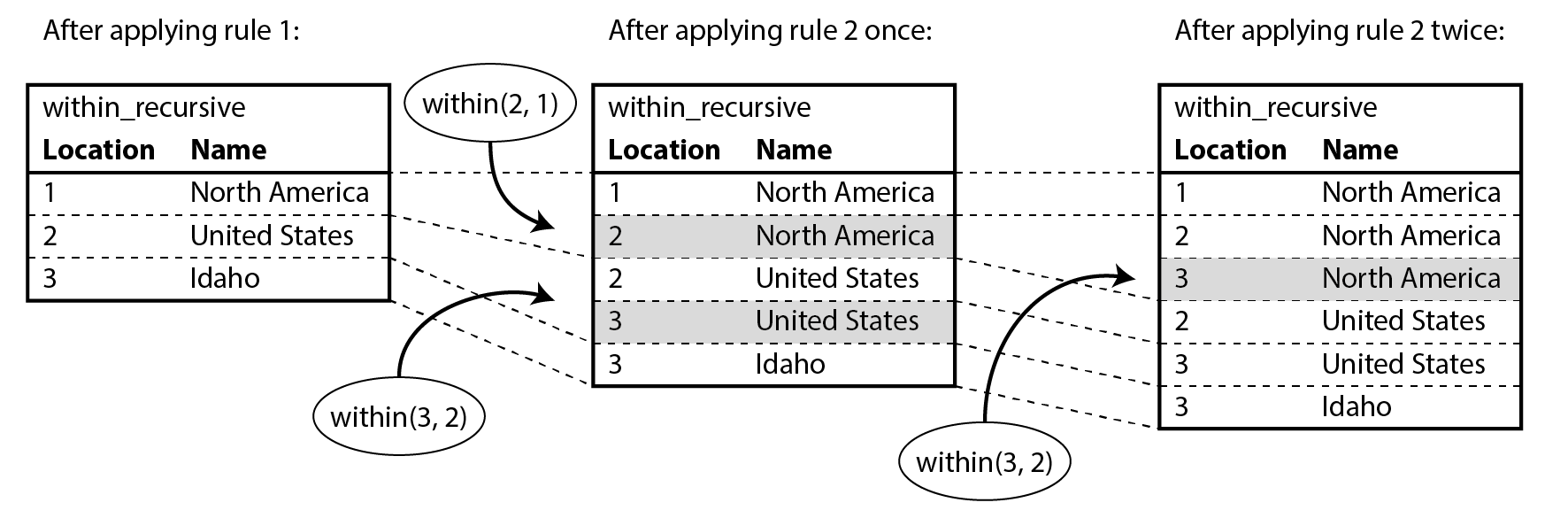
Figure 3-7 Determining that Idaho is in North America, using the Datalog rules from Example 3-12.

Now rule 3 can find people who were born in some location BornIn and live in some location LivingIn. Rule 4 invokes rule 3 with BornIn = 'United States' and LivingIn = 'Europe', and returns only the names of the people who match the search. By querying the contents of the virtual us_to_europe table, the Datalog system finally gets the same answer as in the earlier Cypher and SPARQL queries.

The Datalog approach requires a different kind of thinking compared to the other query languages discussed in this chapter. It allows complex queries to be built up rule by rule, with one rule referring to other rules, similarly to the way that you break down code into functions that call each other. Just like functions can be recursive, Datalog rules can also invoke themselves, like rule 2 in Example 3-12, which enables graph traversals in Datalog queries.

GraphQL

GraphQL is a query language that, by design, is much more restrictive than the other query languages we have seen in this chapter. The purpose of GraphQL is to allow client software running on a user’s device (such as a mobile app or a JavaScript web app frontend) to request a JSON document with a particular structure, containing the fields necessary for rendering its user interface. GraphQL interfaces allow developers to rapidly change queries in client code without changing server-side APIs.

GraphQL’s flexibility comes at a cost. Organizations that adopt GraphQL often need tooling to convert GraphQL queries into requests to internal services, which often use REST or gRPC (see Chapter 5). Authorization, rate limiting, and performance challenges are additional concerns ⁶¹. GraphQL’s query language is also limited since GraphQL come from an untrusted source. The language does not allow anything that could be expensive to execute, since otherwise users could perform denial-of-service attacks on a server by running lots of expensive queries. In particular, GraphQL does not allow recursive queries (unlike Cypher, SPARQL, SQL, or Datalog), and it does not allow arbitrary search conditions such as “find people who were born in the US and are now living in Europe” (unless the service owners specifically choose to offer such search functionality).

Nevertheless, GraphQL is useful. Example 3-13 shows how you might implement a group chat application such as Discord or Slack using GraphQL. The query requests all the channels that the user has access to, including the channel name and the 50 most recent messages in each channel. For each message it requests the timestamp, the message content, and the name and profile picture URL for the sender of the message. Moreover, if a message is a reply to another message, the query also requests the sender name and the content of the message it is replying to (which might be rendered in a smaller font above the reply, in order to provide some context).

Example 3-13. Example GraphQL query for a group chat application

query ChatApp {
    channels {
        name
        recentMessages(latest: 50) {
            timestamp
            content
        sender {
            fullName
            imageUrl
        }
    replyTo {
        content
        sender {
            fullName
        }
    }
    }
    }
}

Example 3-14 shows what a response to the query in Example 3-13 might look like. The response is a JSON document that mirrors the structure of the query: it contains exactly those attributes that were requested, no more and no less. This approach has the advantage that the server does not need to know which attributes the client requires in order to render the user interface; instead, the client can simply request what it needs. For example, this query does not request a profile picture URL for the sender of the replyTo message, but if the user interface were changed to add that profile picture, it would be easy for the client to add the required imageUrl attribute to the query without changing the server.

Example 3-14. A possible response to the query in Example 3-13

{
"data": {
    "channels": [
        {
        "name": "#general",
        "recentMessages": [
        {
        "timestamp": 1693143014,
        "content": "Hey! How are y'all doing?",
        "sender": {"fullName": "Aaliyah", "imageUrl": "https://..."},
        "replyTo": null
        },
        {
            "timestamp": 1693143024,
            "content": "Great! And you?",
            "sender": {"fullName": "Caleb", "imageUrl": "https://..."},
            "replyTo": {
            "content": "Hey! How are y'all doing?",
            "sender": {"fullName": "Aaliyah"}
        }
},
...

In Example 3-14 the name and image URL of a message sender is embedded directly in the message object. If the same user sends multiple messages, this information is repeated on each message. In principle, it would be possible to reduce this duplication, but GraphQL makes the design choice to accept a larger response size in order to make it simpler to render the user interface based on the data.

The replyTo field is similar: in Example 3-14, the second message is a reply to the first, and the content (“Hey!…”) and sender Aaliyah are duplicated under replyTo. It would be possible to instead return the ID of the message being replied to, but then the client would have to make an additional request to the server if that ID is not among the 50 most recent messages returned. Duplicating the content makes it much simpler to work with the data.

The server’s database can store the data in a more normalized form, and perform the necessary joins to process a query. For example, the server might store a message along with the user ID of the sender and the ID of the message it is replying to; when it receives a query like the one above, the server would then resolve those IDs to find the records they refer to. However, the client can only ask the server to perform joins that are explicitly offered in the GraphQL schema.

Even though the response to a GraphQL query looks similar to a response from a document database, and even though it has “graph” in the name, GraphQL can be implemented on top of any type of database—relational, document, or graph.

Event Sourcing and CQRS

In all the data models we have discussed so far, the data is queried in the same form as it is written—be it JSON documents, rows in tables, or vertices and edges in a graph. However, in complex applications it can sometimes be difficult to find a single data representation that is able to satisfy all the different ways that the data needs to be queried and presented. In such situations, it can be beneficial to write data in one form, and then to derive from it several representations that are optimized for different types of reads.

We previously saw this idea in “Systems of Record and Derived Data”, and ETL (see “Data Warehousing”) is one example of such a derivation process. Now we will take the idea further. If we are going to derive one data representation from another anyway, we can choose different representations that are optimized for writing and for reading, respectively. How would you model your data if you only wanted to optimize it for writing, and if efficient queries were of no concern?

Perhaps the simplest, fastest, and most expressive way of writing data is an event log: every time you want to write some data, you encode it as a self-contained string (perhaps as JSON), including a timestamp, and then append it to a sequence of events. Events in this log are immutable: you never change or delete them, you only ever append more events to the log (which may supersede earlier events). An event can contain arbitrary properties.

Figure 3-8 shows an example that could be taken from a conference management system. A conference can be a complex business domain: not only can individual attendees register and pay by card, but companies can also order seats in bulk, pay by invoice, and then later assign the seats to individual people. Some number of seats may be reserved for speakers, sponsors, volunteer helpers, and so on. Reservations may also be cancelled, and meanwhile, the conference organizer might change the capacity of the event by moving it to a different room. With all of this going on, simply calculating the number of available seats becomes a challenging query.

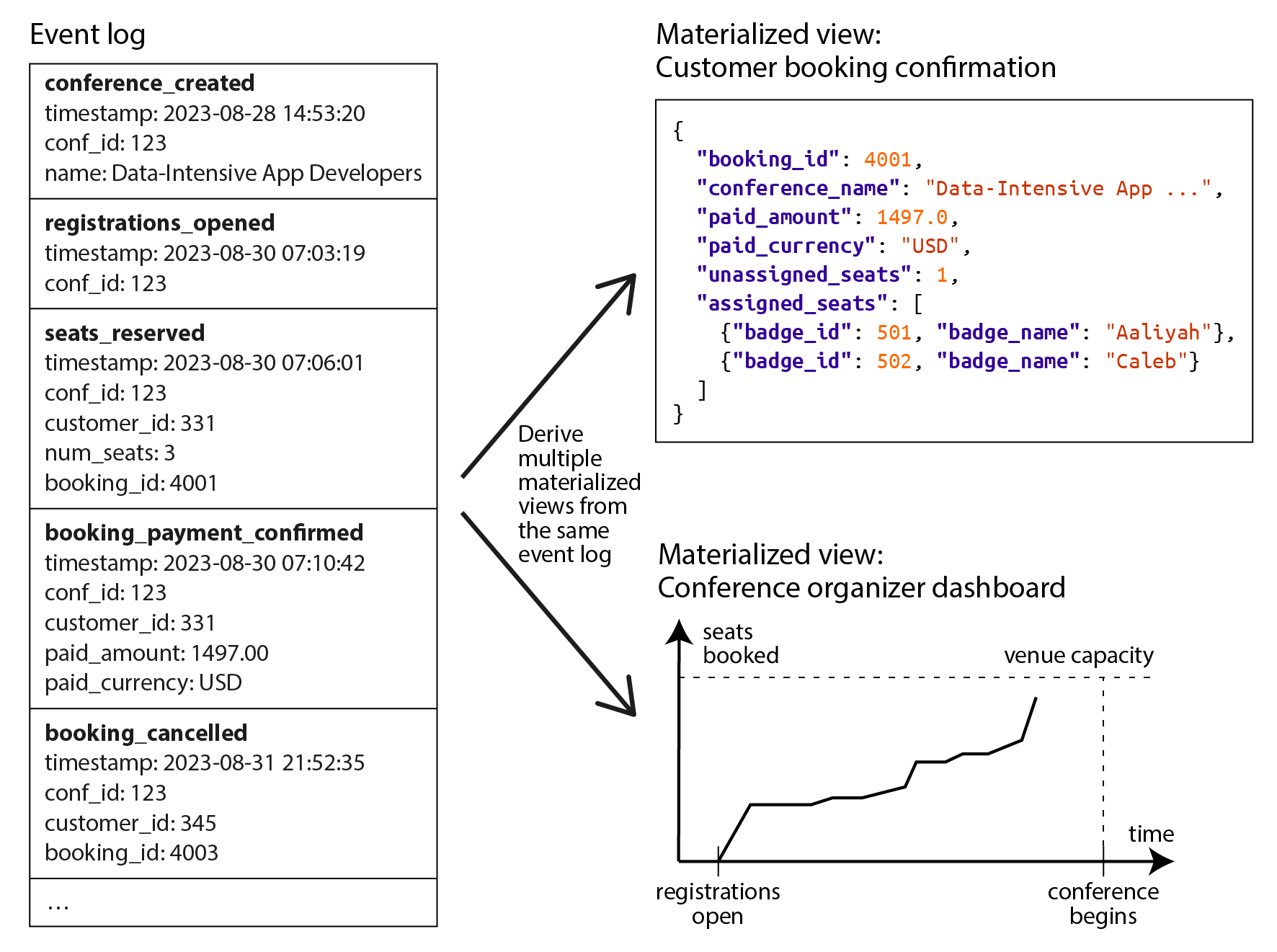
Figure 3-8 Using a log of immutable events as source of truth, and deriving materialized views from it.

In Figure 3-8, every change to the state of the conference (such as the organizer opening registrations, or attendees making and cancelling registrations) is first stored as an event. Whenever an event is appended to the log, several materialized views (also known as projections or read models) are also updated to reflect the effect of that event. In the conference example, there might be one materialized view that collects all information related to the status of each booking, another that computes charts for the conference organizer’s dashboard, and a third that generates files for the printer that produces the attendees’ badges.

The idea of using events as the source of truth, and expressing every state change as an event, is known as event sourcing ⁶² ⁶³. The principle of maintaining separate read-optimized representations and deriving them from the write-optimized representation is called command query responsibility segregation (CQRS) ⁶⁴. These terms originated in the domain-driven design (DDD) community, although similar ideas have been around for a long time, for example in state machine replication (see “Using shared logs”).

When a request from a user comes in, it is called a command, and it first needs to be validated. Only once the command has been executed and it has been determined to be valid (e.g., there were enough available seats for a requested reservation), it becomes a fact, and the corresponding event is added to the log. Consequently, the event log should contain only valid events, and a consumer of the event log that builds a materialized view is not allowed to reject an event.

When modelling your data in an event sourcing style, it is recommended that you name your events in the past tense (e.g., “the seats were booked”), because an event is a record of the fact that something has happened in the past. Even if the user later decides to change or cancel, the fact remains true that they formerly held a booking, and the change or cancellation is a separate event that is added later.

A similarity between event sourcing and a star schema fact table, as discussed in “Stars and Snowflakes: Schemas for Analytics”, is that both are collections of events that happened in the past. However, rows in a fact table all have the same set of columns, wheras in event sourcing there may be many different event types, each with different properties. Moreover, a fact table is an unordered collection, while in event sourcing the order of events is important: if a booking is first made and then cancelled, processing those events in the wrong order would not make sense.

Event sourcing and CQRS have several advantages:

For the people developing the system, events better communicate the intent of why something happened. For example, it’s easier to understand the event “the booking was cancelled” than “the active column on row 4001 of the bookings table was set to false, three rows associated with that booking were deleted from the seat_assignments table, and a row representing the refund was inserted into the payments table”. Those row modifications may still happen when a materialized view processes the cancellation event, but when they are driven by an event, the reason for the updates becomes much clearer.
A key principle of event sourcing is that the materialized views are derived from the event log in a reproducible way: you should always be able to delete the materialized views and recompute them by processing the same events in the same order, using the same code. If there was a bug in the view maintenance code, you can just delete the view and recompute it with the new code. It’s also easier to find the bug because you can re-run the view maintenance code as often as you like and inspect its behavior.
You can have multiple materialized views that are optimized for the particular queries that your application requires. They can be stored either in the same database as the events or a different one, depending on your needs. They can use any data model, and they can be denormalized for fast reads. You can even keep a view only in memory and avoid persisting it, as long as it’s okay to recompute the view from the event log whenever the service restarts.
If you decide you want to present the existing information in a new way, it is easy to build a new materialized view from the existing event log. You can also evolve the system to support new features by adding new types of events, or new properties to existing event types (any older events remain unmodified). You can also chain new behaviors off existing events (for example, when a conference attendee cancels, their seat could be offered to the next person on the waiting list).
If an event was written in error you can delete it again, and then you can rebuild the views without the deleted event. On the other hand, in a database where you update and delete data directly, a committed transaction is often difficult to reverse. Event sourcing can therefore reduce the number of irreversible actions in the system, making it easier to change (see “Evolvability: Making Change Easy”).
The event log can also serve as an audit log of everything that happened in the system, which is valuable in regulated industries that require such auditability.

However, event sourcing and CQRS also have downsides:

You need to be careful if external information is involved. For example, say an event contains a price given in one currency, and for one of the views it needs to be converted into another currency. Since the exchange rate may fluctuate, it would be problematic to fetch the exchange rate from an external source when processing the event, since you would get a different result if you recompute the materialized view on another date. To make the event processing logic deterministic, you either need to include the exchange rate in the event itself, or have a way of querying the historical exchange rate at the timestamp indicated in the event, ensuring that this query always returns the same result for the same timestamp.
The requirement that events are immutable creates problems if events contain personal data from users, since users may exercise their right (e.g., under the GDPR) to request deletion of their data. If the event log is on a per-user basis, you can just delete the whole log for that user, but that doesn’t work if your event log contains events relating to multiple users. You can try storing the personal data outside of the actual event, or encrypting it with a key that you can later choose to delete, but that also makes it harder to recompute derived state when needed.
Reprocessing events requires care if there are externally visible side-effects—for example, you probably don’t want to resend confirmation emails every time you rebuild a materialized view.

You can implement event sourcing on top of any database, but there are also some systems that are specifically designed to support this pattern, such as EventStoreDB, MartenDB (based on PostgreSQL), and Axon Framework. You can also use message brokers such as Apache Kafka to store the event log, and stream processors can keep the materialized views up-to-date; we will return to these topics in “Change data capture versus event sourcing”.

The only important requirement is that the event storage system must guarantee that all materialized views process the events in exactly the same order as they appear in the log; as we shall see in Chapter 10, this is not always easy to achieve in a distributed system.

Dataframes, Matrices, and Arrays

The data models we have seen so far in this chapter are generally used for both transaction processing and analytics purposes (see “Analytical versus Operational Systems”). There are also some data models that you are likely to encounter in an analytical or scientific context, but that rarely feature in OLTP systems: dataframes and multidimensional arrays of numbers such as matrices.

Dataframes are a data model supported by the R language, the Pandas library for Python, Apache Spark, ArcticDB, Dask, and other systems. They are a popular tool for data scientists preparing data for training machine learning models, but they are also widely used for data exploration, statistical data analysis, data visualization, and similar purposes.

At first glance, a dataframe is similar to a table in a relational database or a spreadsheet. It supports relational-like operators that perform bulk operations on the contents of the dataframe: for example, applying a function to all of the rows, filtering the rows based on some condition, grouping rows by some columns and aggregating other columns, and joining the rows in one dataframe with another dataframe based on some key (what a relational database calls join is typically called merge on dataframes).

Instead of a declarative query such as SQL, a dataframe is typically manipulated through a series of commands that modify its structure and content. This matches the typical workflow of data scientists, who incrementally “wrangle” the data into a form that allows them to find answers to the questions they are asking. These manipulations usually take place on the data scientist’s private copy of the dataset, often on their local machine, although the end result may be shared with other users.

Dataframe APIs also offer a wide variety of operations that go far beyond what relational databases offer, and the data model is often used in ways that are very different from typical relational data modelling ⁶⁵. For example, a common use of dataframes is to transform data from a relational-like representation into a matrix or multidimensional array representation, which is the form that many machine learning algorithms expect of their input.

A simple example of such a transformation is shown in Figure 3-9. On the left we have a relational table of how different users have rated various movies (on a scale of 1 to 5), and on the right the data has been transformed into a matrix where each column is a movie and each row is a user (similarly to a pivot table in a spreadsheet). The matrix is sparse, which means there is no data for many user-movie combinations, but this is fine. This matrix may have many thousands of columns and would therefore not fit well in a relational database, but dataframes and libraries that offer sparse arrays (such as NumPy for Python) can handle such data easily.

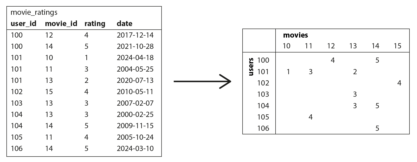
Figure 3-9 Transforming a relational database of movie ratings into a matrix representation.

A matrix can only contain numbers, and various techniques are used to transform non-numerical data into numbers in the matrix. For example:

Dates (which are omitted from the example matrix in Figure 3-9) could be scaled to be floating-point numbers within some suitable range.
For columns that can only take one of a small, fixed set of values (for example, the genre of a movie in a database of movies), a one-hot encoding is often used: we create a column for each possible value (one for “comedy”, one for “drama”, one for “horror”, etc.), and for each row representing a movie, we put a 1 in the column corresponding to the genre of that movie, and a 0 in all the other columns. This representation also easily generalizes to movies that fit within several genres.

Once the data is in the form of a matrix of numbers, it is amenable to linear algebra operations, which form the basis of many machine learning algorithms. For example, the data in Figure 3-9 could be a part of a system for recommending movies that the user may like. Dataframes are flexible enough to allow data to be gradually evolved from a relational form into a matrix representation, while giving the data scientist control over the representation that is most suitable for achieving the goals of the data analysis or model training process.

There are also databases such as TileDB ⁶⁶ that specialize in storing large multidimensional arrays of numbers; they are called array databases and are most commonly used for scientific datasets such as geospatial measurements (raster data on a regularly spaced grid), medical imaging, or observations from astronomical telescopes ⁶⁷. Dataframes are also used in the financial industry for representing time series data, such as the prices of assets and trades over time ⁶⁸.

Summary

Data models are a huge subject, and in this chapter we have taken a quick look at a broad variety of different models. We didn’t have space to go into all the details of each model, but hopefully the overview has been enough to whet your appetite to find out more about the model that best fits your application’s requirements.

The relational model, despite being more than half a century old, remains an important data model for many applications—especially in data warehousing and business analytics, where relational star or snowflake schemas and SQL queries are ubiquitous. However, several alternatives to relational data have also become popular in other domains:

The document model targets use cases where data comes in self-contained JSON documents, and where relationships between one document and another are rare.
Graph data models go in the opposite direction, targeting use cases where anything is potentially related to everything, and where queries potentially need to traverse multiple hops to find the data of interest (which can be expressed using recursive queries in Cypher, SPARQL, or Datalog).
Dataframes generalize relational data to large numbers of columns, and thereby provide a bridge between databases and the multidimensional arrays that form the basis of much machine learning, statistical data analysis, and scientific computing.

To some degree, one model can be emulated in terms of another model—for example, graph data can be represented in a relational database—but the result can be awkward, as we saw with the support for recursive queries in SQL.

Various specialist databases have therefore been developed for each data model, providing query languages and storage engines that are optimized for a particular model. However, there is also a trend for databases to expand into neighboring niches by adding support for other data models: for example, relational databases have added support for document data in the form of JSON columns, document databases have added relational-like joins, and support for graph data within SQL is gradually improving.

Another model we discussed is event sourcing, which represents data as an append-only log of immutable events, and which can be advantageous for modeling activities in complex business domains. An append-only log is good for writing data (as we shall see in Chapter 4); in order to support efficient queries, the event log is translated into read-optimized materialized views through CQRS.

One thing that non-relational data models have in common is that they typically don’t enforce a schema for the data they store, which can make it easier to adapt applications to changing requirements. However, your application most likely still assumes that data has a certain structure; it’s just a question of whether the schema is explicit (enforced on write) or implicit (assumed on read).

Although we have covered a lot of ground, there are still data models left unmentioned. To give just a few brief examples:

Researchers working with genome data often need to perform sequence-similarity searches, which means taking one very long string (representing a DNA molecule) and matching it against a large database of strings that are similar, but not identical. None of the databases described here can handle this kind of usage, which is why researchers have written specialized genome database software like GenBank ⁶⁹.
Many financial systems use ledgers with double-entry accounting as their data model. This type of data can be represented in relational databases, but there are also databases such as TigerBeetle that specialize in this data model. Cryptocurrencies and blockchains are typically based on distributed ledgers, which also have value transfer built into their data model.
Full-text search is arguably a kind of data model that is frequently used alongside databases. Information retrieval is a large specialist subject that we won’t cover in great detail in this book, but we’ll touch on search indexes and vector search in “Full-Text Search”.

We have to leave it there for now. In the next chapter we will discuss some of the trade-offs that come into play when implementing the data models described in this chapter.

References

Jamie Brandon. Unexplanations: query optimization works because sql is declarative. scattered-thoughts.net, February 2024. Archived at perma.cc/P6W2-WMFZ ↩︎
Joseph M. Hellerstein. The Declarative Imperative: Experiences and Conjectures in Distributed Logic. Tech report UCB/EECS-2010-90, Electrical Engineering and Computer Sciences, University of California at Berkeley, June 2010. Archived at perma.cc/K56R-VVQM ↩︎
Edgar F. Codd. A Relational Model of Data for Large Shared Data Banks. Communications of the ACM, volume 13, issue 6, pages 377–387, June 1970. doi:10.1145/362384.362685 ↩︎ ↩︎
Michael Stonebraker and Joseph M. Hellerstein. What Goes Around Comes Around. In Readings in Database Systems, 4th edition, MIT Press, pages 2–41, 2005. ISBN: 9780262693141 ↩︎
Markus Winand. Modern SQL: Beyond Relational. modern-sql.com, 2015. Archived at perma.cc/D63V-WAPN ↩︎
Martin Fowler. OrmHate. martinfowler.com, May 2012. Archived at perma.cc/VCM8-PKNG ↩︎
Vlad Mihalcea. N+1 query problem with JPA and Hibernate. vladmihalcea.com, January 2023. Archived at perma.cc/79EV-TZKB ↩︎
Jens Schauder. This is the Beginning of the End of the N+1 Problem: Introducing Single Query Loading. spring.io, August 2023. Archived at perma.cc/6V96-R333 ↩︎
William Zola. 6 Rules of Thumb for MongoDB Schema Design. mongodb.com, June 2014. Archived at perma.cc/T2BZ-PPJB ↩︎ ↩︎
Sidney Andrews and Christopher McClister. Data modeling in Azure Cosmos DB. learn.microsoft.com, February 2023. Archived at archive.org ↩︎
Raffi Krikorian. Timelines at Scale. At QCon San Francisco, November 2012. Archived at perma.cc/V9G5-KLYK ↩︎ ↩︎
Ralph Kimball and Margy Ross. The Data Warehouse Toolkit: The Definitive Guide to Dimensional Modeling, 3rd edition. John Wiley & Sons, July 2013. ISBN: 9781118530801 ↩︎ ↩︎
Michael Kaminsky. Data warehouse modeling: Star schema vs. OBT. fivetran.com, August 2022. Archived at perma.cc/2PZK-BFFP ↩︎
Joe Nelson. User-defined Order in SQL. begriffs.com, March 2018. Archived at perma.cc/GS3W-F7AD ↩︎
Evan Wallace. Realtime Editing of Ordered Sequences. figma.com, March 2017. Archived at perma.cc/K6ER-CQZW ↩︎
David Greenspan. Implementing Fractional Indexing. observablehq.com, October 2020. Archived at perma.cc/5N4R-MREN ↩︎
Martin Fowler. Schemaless Data Structures. martinfowler.com, January 2013. ↩︎
Amr Awadallah. Schema-on-Read vs. Schema-on-Write. At Berkeley EECS RAD Lab Retreat, Santa Cruz, CA, May 2009. Archived at perma.cc/DTB2-JCFR ↩︎
Martin Odersky. The Trouble with Types. At Strange Loop, September 2013. Archived at perma.cc/85QE-PVEP ↩︎
Conrad Irwin. MongoDB—Confessions of a PostgreSQL Lover. At HTML5DevConf, October 2013. Archived at perma.cc/C2J6-3AL5 ↩︎
Percona Toolkit Documentation: pt-online-schema-change. docs.percona.com, 2023. Archived at perma.cc/9K8R-E5UH ↩︎
Shlomi Noach. gh-ost: GitHub’s Online Schema Migration Tool for MySQL. github.blog, August 2016. Archived at perma.cc/7XAG-XB72 ↩︎
Shayon Mukherjee. pg-osc: Zero downtime schema changes in PostgreSQL. shayon.dev, February 2022. Archived at perma.cc/35WN-7WMY ↩︎
Carlos Pérez-Aradros Herce. Introducing pgroll: zero-downtime, reversible, schema migrations for Postgres. xata.io, October 2023. Archived at archive.org ↩︎
James C. Corbett, Jeffrey Dean, Michael Epstein, Andrew Fikes, Christopher Frost, JJ Furman, Sanjay Ghemawat, Andrey Gubarev, Christopher Heiser, Peter Hochschild, Wilson Hsieh, Sebastian Kanthak, Eugene Kogan, Hongyi Li, Alexander Lloyd, Sergey Melnik, David Mwaura, David Nagle, Sean Quinlan, Rajesh Rao, Lindsay Rolig, Dale Woodford, Yasushi Saito, Christopher Taylor, Michal Szymaniak, and Ruth Wang. Spanner: Google’s Globally-Distributed Database. At 10th USENIX Symposium on Operating System Design and Implementation (OSDI), October 2012. ↩︎
Donald K. Burleson. Reduce I/O with Oracle Cluster Tables. dba-oracle.com. Archived at perma.cc/7LBJ-9X2C ↩︎
Fay Chang, Jeffrey Dean, Sanjay Ghemawat, Wilson C. Hsieh, Deborah A. Wallach, Mike Burrows, Tushar Chandra, Andrew Fikes, and Robert E. Gruber. Bigtable: A Distributed Storage System for Structured Data. At 7th USENIX Symposium on Operating System Design and Implementation (OSDI), November 2006. ↩︎
Priscilla Walmsley. XQuery, 2nd Edition. O’Reilly Media, December 2015. ISBN: 9781491915080 ↩︎
Paul C. Bryan, Kris Zyp, and Mark Nottingham. JavaScript Object Notation (JSON) Pointer. RFC 6901, IETF, April 2013. ↩︎
Stefan Gössner, Glyn Normington, and Carsten Bormann. JSONPath: Query Expressions for JSON. RFC 9535, IETF, February 2024. ↩︎
Michael Stonebraker and Andrew Pavlo. What Goes Around Comes Around… And Around…. ACM SIGMOD Record, volume 53, issue 2, pages 21–37. doi:10.1145/3685980.3685984 ↩︎
Lawrence Page, Sergey Brin, Rajeev Motwani, and Terry Winograd. The PageRank Citation Ranking: Bringing Order to the Web. Technical Report 1999-66, Stanford University InfoLab, November 1999. Archived at perma.cc/UML9-UZHW ↩︎
Nathan Bronson, Zach Amsden, George Cabrera, Prasad Chakka, Peter Dimov, Hui Ding, Jack Ferris, Anthony Giardullo, Sachin Kulkarni, Harry Li, Mark Marchukov, Dmitri Petrov, Lovro Puzar, Yee Jiun Song, and Venkat Venkataramani. TAO: Facebook’s Distributed Data Store for the Social Graph. At USENIX Annual Technical Conference (ATC), June 2013. ↩︎
Natasha Noy, Yuqing Gao, Anshu Jain, Anant Narayanan, Alan Patterson, and Jamie Taylor. Industry-Scale Knowledge Graphs: Lessons and Challenges. Communications of the ACM, volume 62, issue 8, pages 36–43, August 2019. doi:10.1145/3331166 ↩︎
Xiyang Feng, Guodong Jin, Ziyi Chen, Chang Liu, and Semih Salihoğlu. KÙZU Graph Database Management System. At 3th Annual Conference on Innovative Data Systems Research (CIDR 2023), January 2023. ↩︎ ↩︎
Maciej Besta, Emanuel Peter, Robert Gerstenberger, Marc Fischer, Michał Podstawski, Claude Barthels, Gustavo Alonso, Torsten Hoefler. Demystifying Graph Databases: Analysis and Taxonomy of Data Organization, System Designs, and Graph Queries. arxiv.org, October 2019. ↩︎ ↩︎
Apache TinkerPop 3.6.3 Documentation. tinkerpop.apache.org, May 2023. Archived at perma.cc/KM7W-7PAT ↩︎
Nadime Francis, Alastair Green, Paolo Guagliardo, Leonid Libkin, Tobias Lindaaker, Victor Marsault, Stefan Plantikow, Mats Rydberg, Petra Selmer, and Andrés Taylor. Cypher: An Evolving Query Language for Property Graphs. At International Conference on Management of Data (SIGMOD), pages 1433–1445, May 2018. doi:10.1145/3183713.3190657 ↩︎
Emil Eifrem. Twitter correspondence, January 2014. Archived at perma.cc/WM4S-BW64 ↩︎
Francesco Tisiot. Explore the new SEARCH and CYCLE features in PostgreSQL® 14. aiven.io, December 2021. Archived at perma.cc/J6BT-83UZ ↩︎
Gaurav Goel. Understanding Hierarchies in Oracle. towardsdatascience.com, May 2020. Archived at perma.cc/5ZLR-Q7EW ↩︎
Alin Deutsch, Nadime Francis, Alastair Green, Keith Hare, Bei Li, Leonid Libkin, Tobias Lindaaker, Victor Marsault, Wim Martens, Jan Michels, Filip Murlak, Stefan Plantikow, Petra Selmer, Oskar van Rest, Hannes Voigt, Domagoj Vrgoč, Mingxi Wu, and Fred Zemke. Graph Pattern Matching in GQL and SQL/PGQ. At International Conference on Management of Data (SIGMOD), pages 2246–2258, June 2022. doi:10.1145/3514221.3526057 ↩︎
Alastair Green. SQL… and now GQL. opencypher.org, September 2019. Archived at perma.cc/AFB2-3SY7 ↩︎
Alin Deutsch, Yu Xu, and Mingxi Wu. Seamless Syntactic and Semantic Integration of Query Primitives over Relational and Graph Data in GSQL. tigergraph.com, November 2018. Archived at perma.cc/JG7J-Y35X ↩︎
Oskar van Rest, Sungpack Hong, Jinha Kim, Xuming Meng, and Hassan Chafi. PGQL: a property graph query language. At 4th International Workshop on Graph Data Management Experiences and Systems (GRADES), June 2016. doi:10.1145/2960414.2960421 ↩︎
Amazon Web Services. Neptune Graph Data Model. Amazon Neptune User Guide, docs.aws.amazon.com. Archived at perma.cc/CX3T-EZU9 ↩︎
Cognitect. Datomic Data Model. Datomic Cloud Documentation, docs.datomic.com. Archived at perma.cc/LGM9-LEUT ↩︎
David Beckett and Tim Berners-Lee. Turtle – Terse RDF Triple Language. W3C Team Submission, March 2011. ↩︎
Sinclair Target. Whatever Happened to the Semantic Web? twobithistory.org, May 2018. Archived at perma.cc/M8GL-9KHS ↩︎
Gavin Mendel-Gleason. The Semantic Web is Dead – Long Live the Semantic Web! terminusdb.com, August 2022. Archived at perma.cc/G2MZ-DSS3 ↩︎
Manu Sporny. JSON-LD and Why I Hate the Semantic Web. manu.sporny.org, January 2014. Archived at perma.cc/7PT4-PJKF ↩︎
University of Michigan Library. Biomedical Ontologies and Controlled Vocabularies, guides.lib.umich.edu/ontology. Archived at perma.cc/Q5GA-F2N8 ↩︎
Facebook. The Open Graph protocol, ogp.me. Archived at perma.cc/C49A-GUSY ↩︎
Matt Haughey. Everything you ever wanted to know about unfurling but were afraid to ask /or/ How to make your site previews look amazing in Slack. medium.com, November 2015. Archived at perma.cc/C7S8-4PZN ↩︎
W3C RDF Working Group. Resource Description Framework (RDF). w3.org, February 2004. ↩︎
Steve Harris, Andy Seaborne, and Eric Prud’hommeaux. SPARQL 1.1 Query Language. W3C Recommendation, March 2013. ↩︎
Todd J. Green, Shan Shan Huang, Boon Thau Loo, and Wenchao Zhou. Datalog and Recursive Query Processing. Foundations and Trends in Databases, volume 5, issue 2, pages 105–195, November 2013. doi:10.1561/1900000017 ↩︎
Stefano Ceri, Georg Gottlob, and Letizia Tanca. What You Always Wanted to Know About Datalog (And Never Dared to Ask). IEEE Transactions on Knowledge and Data Engineering, volume 1, issue 1, pages 146–166, March 1989. doi:10.1109/69.43410 ↩︎
Serge Abiteboul, Richard Hull, and Victor Vianu. Foundations of Databases. Addison-Wesley, 1995. ISBN: 9780201537710, available online at webdam.inria.fr/Alice ↩︎
Scott Meyer, Andrew Carter, and Andrew Rodriguez. LIquid: The soul of a new graph database, Part 2. engineering.linkedin.com, September 2020. Archived at perma.cc/K9M4-PD6Q ↩︎
Matt Bessey. Why, after 6 years, I’m over GraphQL. bessey.dev, May 2024. Archived at perma.cc/2PAU-JYRA ↩︎
Dominic Betts, Julián Domínguez, Grigori Melnik, Fernando Simonazzi, and Mani Subramanian. Exploring CQRS and Event Sourcing. Microsoft Patterns & Practices, July 2012. ISBN: 1621140164, archived at perma.cc/7A39-3NM8 ↩︎
Greg Young. CQRS and Event Sourcing. At Code on the Beach, August 2014. ↩︎
Greg Young. CQRS Documents. cqrs.wordpress.com, November 2010. Archived at perma.cc/X5R6-R47F ↩︎
Devin Petersohn, Stephen Macke, Doris Xin, William Ma, Doris Lee, Xiangxi Mo, Joseph E. Gonzalez, Joseph M. Hellerstein, Anthony D. Joseph, and Aditya Parameswaran. Towards Scalable Dataframe Systems. Proceedings of the VLDB Endowment, volume 13, issue 11, pages 2033–2046. doi:10.14778/3407790.3407807 ↩︎
Stavros Papadopoulos, Kushal Datta, Samuel Madden, and Timothy Mattson. The TileDB Array Data Storage Manager. Proceedings of the VLDB Endowment, volume 10, issue 4, pages 349–360, November 2016. doi:10.14778/3025111.3025117 ↩︎
Florin Rusu. Multidimensional Array Data Management. Foundations and Trends in Databases, volume 12, numbers 2–3, pages 69–220, February 2023. doi:10.1561/1900000069 ↩︎
Ed Targett. Bloomberg, Man Group team up to develop open source “ArcticDB” database. thestack.technology, March 2023. Archived at perma.cc/M5YD-QQYV ↩︎
Dennis A. Benson, Ilene Karsch-Mizrachi, David J. Lipman, James Ostell, and David L. Wheeler. GenBank. Nucleic Acids Research, volume 36, database issue, pages D25–D30, December 2007. doi:10.1093/nar/gkm929 ↩︎

4. Storage and Retrieval

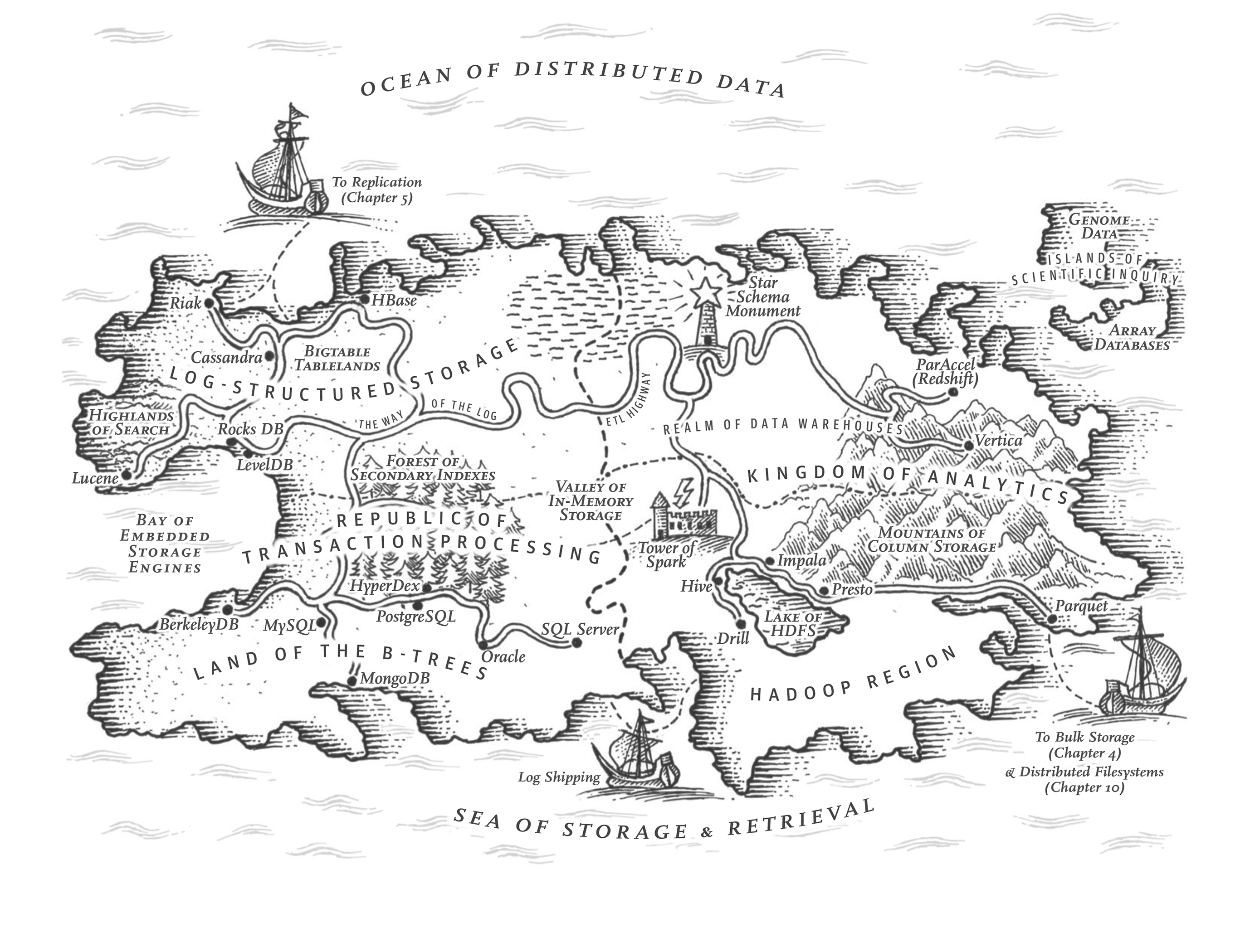
One of the miseries of life is that everybody names things a little bit wrong. And so it makes everything a little harder to understand in the world than it would be if it were named differently. A computer does not primarily compute in the sense of doing arithmetic. […] They primarily are filing systems.

Richard Feynman, Idiosyncratic Thinking seminar (1985)

On the most fundamental level, a database needs to do two things: when you give it some data, it should store the data, and when you ask it again later, it should give the data back to you.

In Chapter 3 we discussed data models and query languages—i.e., the format in which you give the database your data, and the interface through which you can ask for it again later. In this chapter we discuss the same from the database’s point of view: how the database can store the data that you give it, and how it can find the data again when you ask for it.

Why should you, as an application developer, care how the database handles storage and retrieval internally? You’re probably not going to implement your own storage engine from scratch, but you do need to select a storage engine that is appropriate for your application, from the many that are available. In order to configure a storage engine to perform well on your kind of workload, you need to have a rough idea of what the storage engine is doing under the hood.

In particular, there is a big difference between storage engines that are optimized for transactional workloads (OLTP) and those that are optimized for analytics (we introduced this distinction in “Analytical versus Operational Systems”). This chapter starts by examining two families of storage engines for OLTP: log-structured storage engines that write out immutable data files, and storage engines such as B-trees that update data in-place. These structures are used for both key-value storage as well as secondary indexes.

Later in “Data Storage for Analytics” we’ll discuss a family of storage engines that is optimized for analytics, and in “Multidimensional and Full-Text Indexes” we’ll briefly look at indexes for more advanced queries, such as text retrieval.

Storage and Indexing for OLTP

Consider the world’s simplest database, implemented as two Bash functions:

#!/bin/bash

db_set () {
  echo "$1,$2" >> database
}

db_get () {
  grep "^$1," database | sed -e "s/^$1,//" | tail -n 1
}

These two functions implement a key-value store. You can call db_set key value, which will store key and value in the database. The key and value can be (almost) anything you like—for example, the value could be a JSON document. You can then call db_get key, which looks up the most recent value associated with that particular key and returns it.

And it works:

$ db_set 12 '{"name":"London","attractions":["Big Ben","London Eye"]}'

$ db_set 42 '{"name":"San Francisco","attractions":["Golden Gate Bridge"]}'

$ db_get 42
{"name":"San Francisco","attractions":["Golden Gate Bridge"]}

The storage format is very simple: a text file where each line contains a key-value pair, separated by a comma (roughly like a CSV file, ignoring escaping issues). Every call to db_set appends to the end of the file. If you update a key several times, old versions of the value are not overwritten—you need to look at the last occurrence of a key in a file to find the latest value (hence the tail -n 1 in db_get):

$ db_set 42 '{"name":"San Francisco","attractions":["Exploratorium"]}'

$ db_get 42
{"name":"San Francisco","attractions":["Exploratorium"]}

$ cat database
12,{"name":"London","attractions":["Big Ben","London Eye"]}
42,{"name":"San Francisco","attractions":["Golden Gate Bridge"]}
42,{"name":"San Francisco","attractions":["Exploratorium"]}

The db_set function actually has pretty good performance for something that is so simple, because appending to a file is generally very efficient. Similarly to what db_set does, many databases internally use a log, which is an append-only data file. Real databases have more issues to deal with (such as handling concurrent writes, reclaiming disk space so that the log doesn’t grow forever, and handling partially written records when recovering from a crash), but the basic principle is the same. Logs are incredibly useful, and we will encounter them several times in this book.

Note

The word log is often used to refer to application logs, where an application outputs text that describes what’s happening. In this book, log is used in the more general sense: an append-only sequence of records on disk. It doesn’t have to be human-readable; it might be binary and intended only for internal use by the database system.

On the other hand, the db_get function has terrible performance if you have a large number of records in your database. Every time you want to look up a key, db_get has to scan the entire database file from beginning to end, looking for occurrences of the key. In algorithmic terms, the cost of a lookup is O(n): if you double the number of records n in your database, a lookup takes twice as long. That’s not good.

In order to efficiently find the value for a particular key in the database, we need a different data structure: an index. In this chapter we will look at a range of indexing structures and see how they compare; the general idea is to structure the data in a particular way (e.g., sorted by some key) that makes it faster to locate the data you want. If you want to search the same data in several different ways, you may need several different indexes on different parts of the data.

An index is an additional structure that is derived from the primary data. Many databases allow you to add and remove indexes, and this doesn’t affect the contents of the database; it only affects the performance of queries. Maintaining additional structures incurs overhead, especially on writes. For writes, it’s hard to beat the performance of simply appending to a file, because that’s the simplest possible write operation. Any kind of index usually slows down writes, because the index also needs to be updated every time data is written.

This is an important trade-off in storage systems: well-chosen indexes speed up read queries, but every index consumes additional disk space and slows down writes, sometimes substantially ¹. For this reason, databases don’t usually index everything by default, but require you—the person writing the application or administering the database—to choose indexes manually, using your knowledge of the application’s typical query patterns. You can then choose the indexes that give your application the greatest benefit, without introducing more overhead on writes than necessary.

Log-Structured Storage

To start, let’s assume that you want to continue storing data in the append-only file written by db_set, and you just want to speed up reads. One way you could do this is by keeping a hash map in memory, in which every key is mapped to the byte offset in the file at which the most recent value for that key can be found, as illustrated in Figure 4-1.

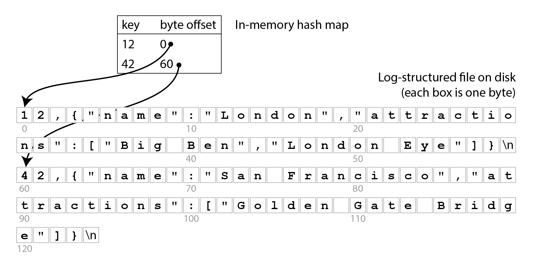
Figure 4-1 Storing a log of key-value pairs in a CSV-like format, indexed with an in-memory hash map.

Whenever you append a new key-value pair to the file, you also update the hash map to reflect the offset of the data you just wrote. When you want to look up a value, you use the hash map to find the offset in the log file, seek to that location, and read the value. If that part of the data file is already in the filesystem cache, a read doesn’t require any disk I/O at all.

This approach is much faster, but it still suffers from several problems:

You never free up disk space occupied by old log entries that have been overwritten; if you keep writing to the database you might run out of disk space.
The hash map is not persisted, so you have to rebuild it when you restart the database—for example, by scanning the whole log file to find the latest byte offset for each key. This makes restarts slow if you have a lot of data.
The hash table must fit in memory. In principle, you could maintain a hash table on disk, but unfortunately it is difficult to make an on-disk hash map perform well. It requires a lot of random access I/O, it is expensive to grow when it becomes full, and hash collisions require fiddly logic ².
Range queries are not efficient. For example, you cannot easily scan over all keys between 10000 and 19999—you’d have to look up each key individually in the hash map.

The SSTable file format

In practice, hash tables are not used very often for database indexes, and instead it is much more common to keep data in a structure that is sorted by key ³. One example of such a structure is a Sorted String Table, or SSTable for short, as shown in Figure 4-2. This file format also stores key-value pairs, but it ensures that they are sorted by key, and each key only appears once in the file.

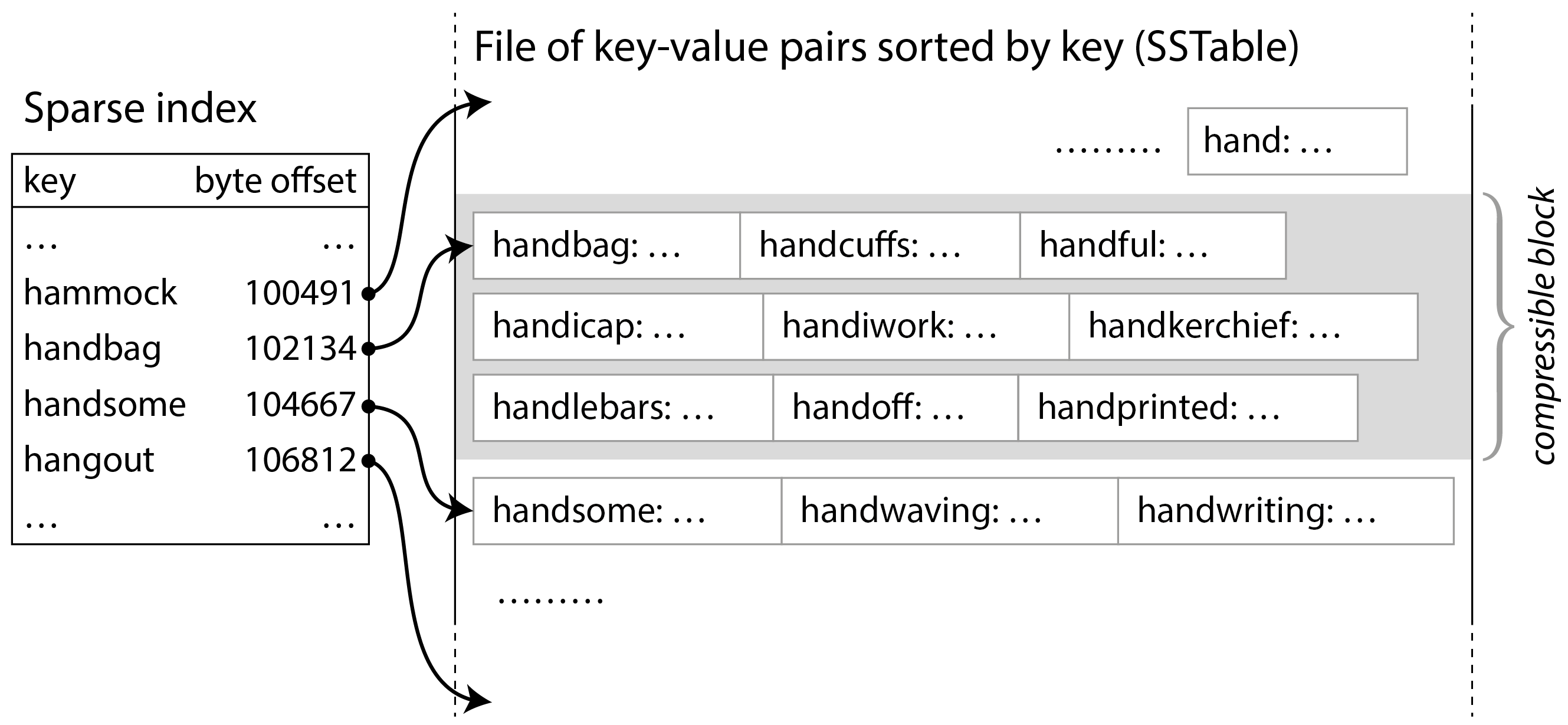
Figure 4-2 An SSTable with a sparse index, allowing queries to jump to the right block.

Now you do not need to keep all the keys in memory: you can group the key-value pairs within an SSTable into blocks of a few kilobytes, and then store the first key of each block in the index. This kind of index, which stores only some of the keys, is called sparse. This index is stored in a separate part of the SSTable, for example using an immutable B-tree, a trie, or another data structure that allows queries to quickly look up a particular key ⁴.

For example, in Figure 4-2, the first key of one block is handbag, and the first key of the next block is handsome. Now say you’re looking for the key handiwork, which doesn’t appear in the sparse index. Because of the sorting you know that handiwork must appear between handbag and handsome. This means you can seek to the offset for handbag and scan the file from there until you find handiwork (or not, if the key is not present in the file). A block of a few kilobytes can be scanned very quickly.

Moreover, each block of records can be compressed (indicated by the shaded area in Figure 4-2). Besides saving disk space, compression also reduces the I/O bandwidth use, at the cost of using a bit more CPU time.

Constructing and merging SSTables

The SSTable file format is better for reading than an append-only log, but it makes writes more difficult. We can’t simply append at the end, because then the file would no longer be sorted (unless the keys happen to be written in ascending order). If we had to rewrite the whole SSTable every time a key is inserted somewhere in the middle, writes would become far too expensive.

We can solve this problem with a log-structured approach, which is a hybrid between an append-only log and a sorted file:

When a write comes in, add it to an in-memory ordered map data structure, such as a red-black tree, skip list ⁵, or trie ⁶. With these data structures, you can insert keys in any order, look them up efficiently, and read them back in sorted order. This in-memory data structure is called the memtable.
When the memtable gets bigger than some threshold—typically a few megabytes—write it out to disk in sorted order as an SSTable file. We call this new SSTable file the most recent segment of the database, and it is stored as a separate file alongside the older segments. Each segment has a separate index of its contents. While the new segment is being written out to disk, the database can continue writing to a new memtable instance, and the old memtable’s memory is freed when the writing of the SSTable is complete.
In order to read the value for some key, first try to find the key in the memtable and the most recent on-disk segment. If it’s not there, look in the next-older segment, etc. until you either find the key or reach the oldest segment. If the key does not appear in any of the segments, it does not exist in the database.
From time to time, run a merging and compaction process in the background to combine segment files and to discard overwritten or deleted values.

Merging segments works similarly to the mergesort algorithm ⁵. The process is illustrated in Figure 4-3: start reading the input files side by side, look at the first key in each file, copy the lowest key (according to the sort order) to the output file, and repeat. If the same key appears in more than one input file, keep only the more recent value. This produces a new merged segment file, also sorted by key, with one value per key, and it uses minimal memory because we can iterate over the SSTables one key at a time.

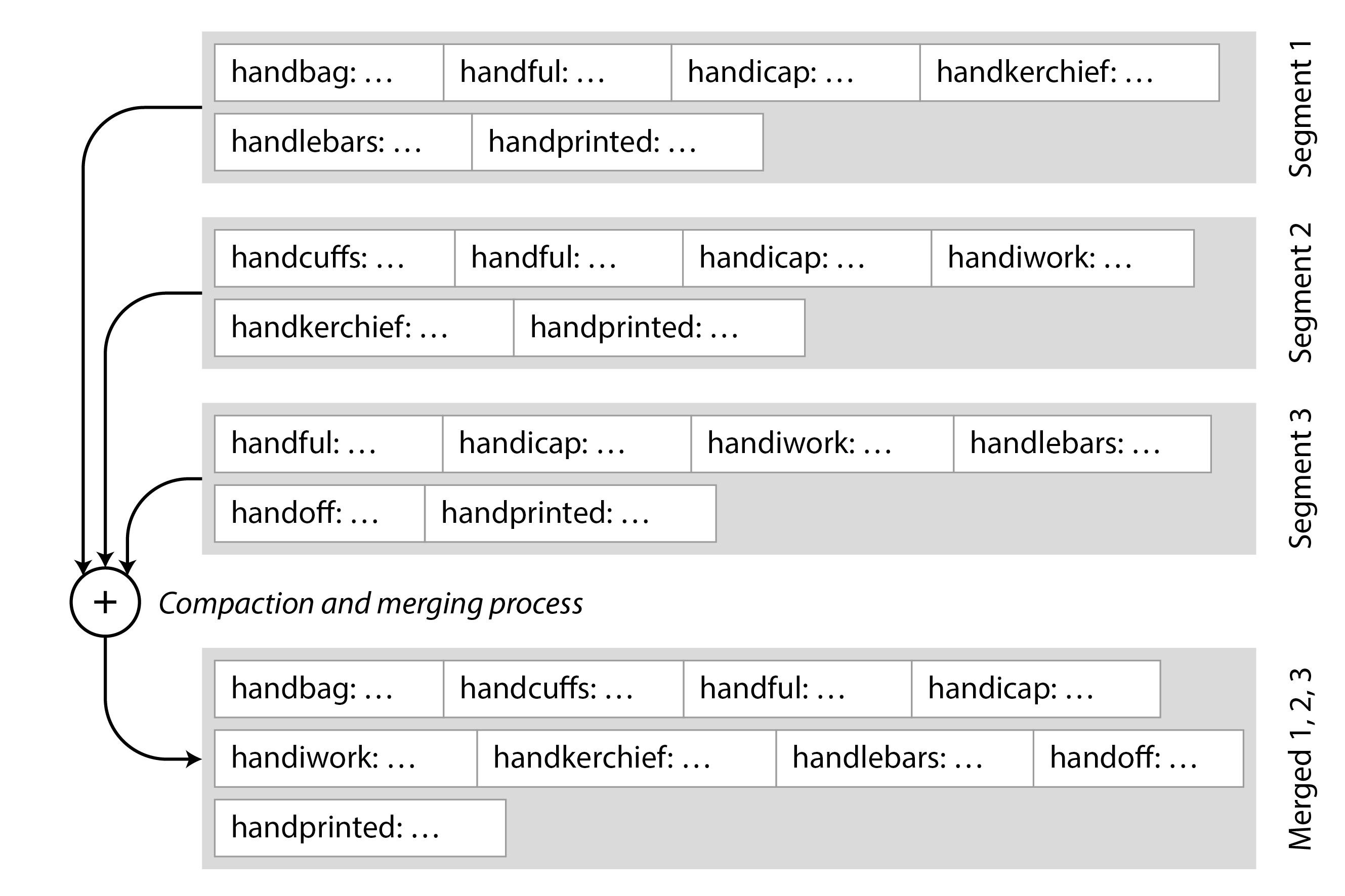
Figure 4-3 Merging several SSTable segments, retaining only the most recent value for each key.

To ensure that the data in the memtable is not lost if the database crashes, the storage engine keeps a separate log on disk to which every write is immediately appended. This log is not sorted by key, but that doesn’t matter, because its only purpose is to restore the memtable after a crash. Every time the memtable has been written out to an SSTable, the corresponding part of the log can be discarded.

If you want to delete a key and its associated value, you have to append a special deletion record called a tombstone to the data file. When log segments are merged, the tombstone tells the merging process to discard any previous values for the deleted key. Once the tombstone is merged into the oldest segment, it can be dropped.

The algorithm described here is essentially what is used in RocksDB ⁷, Cassandra, Scylla, and HBase ⁸, all of which were inspired by Google’s Bigtable paper ⁹ (which introduced the terms SSTable and memtable).

The algorithm was originally published in 1996 under the name Log-Structured Merge-Tree or LSM-Tree ¹⁰, building on earlier work on log-structured filesystems ¹¹. For this reason, storage engines that are based on the principle of merging and compacting sorted files are often called LSM storage engines.

In LSM storage engines, a segment file is written in one pass (either by writing out the memtable or by merging some existing segments), and thereafter it is immutable. The merging and compaction of segments can be done in a background thread, and while it is going on, we can still continue to serve reads using the old segment files. When the merging process is complete, we switch read requests to using the new merged segment instead of the old segments, and then the old segment files can be deleted.

The segment files don’t necessarily have to be stored on local disk: they are also well suited for writing to object storage. SlateDB and Delta Lake ¹². take this approach, for example.

Having immutable segment files also simplifies crash recovery: if a crash happens while writing out the memtable or while merging segments, the database can just delete the unfinished SSTable and start afresh. The log that persists writes to the memtable could contain incomplete records if there was a crash halfway through writing a record, or if the disk was full; these are typically detected by including checksums in the log, and discarding corrupted or incomplete log entries. We will talk more about durability and crash recovery in Chapter 8.

Bloom filters

With LSM storage it can be slow to read a key that was last updated a long time ago, or that does not exist, since the storage engine needs to check several segment files. In order to speed up such reads, LSM storage engines often include a Bloom filter ¹³ in each segment, which provides a fast but approximate way of checking whether a particular key appears in a particular SSTable.

Figure 4-4 shows an example of a Bloom filter containing two keys and 16 bits (in reality, it would contain more keys and more bits). For every key in the SSTable we compute a hash function, producing a set of numbers that are then interpreted as indexes into the array of bits ¹⁴. We set the bits corresponding to those indexes to 1, and leave the rest as 0. For example, the key handbag hashes to the numbers (2, 9, 4), so we set the 2nd, 9th, and 4th bits to 1. The bitmap is then stored as part of the SSTable, along with the sparse index of keys. This takes a bit of extra space, but the Bloom filter is generally small compared to the rest of the SSTable.

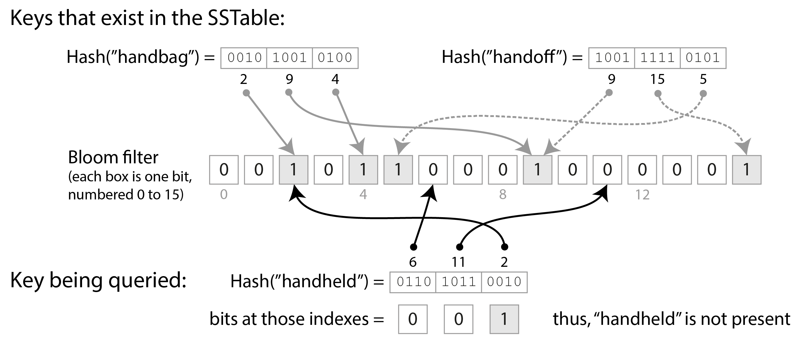
Figure 4-4 A Bloom filter provides a fast, probabilistic check whether a particular key exists in a particular SSTable.

When we want to know whether a key appears in the SSTable, we compute the same hash of that key as before, and check the bits at those indexes. For example, in Figure 4-4, we’re querying the key handheld, which hashes to (6, 11, 2). One of those bits is 1 (namely, bit number 2), while the other two are 0. These checks can be made extremely fast using the bitwise operations that all CPUs support.

If at least one of the bits is 0, we know that the key definitely does not appear in the SSTable. If the bits in the query are all 1, it’s likely that the key is in the SSTable, but it’s also possible that by coincidence all of those bits were set to 1 by other keys. This case when it looks as if a key is present, even though it isn’t, is called a false positive.

The probability of false positives depends on the number of keys, the number of bits set per key, and the total number of bits in the Bloom filter. You can use an online calculator tool to work out the right parameters for your application ¹⁵. As a rule of thumb, you need to allocate 10 bits of Bloom filter space for every key in the SSTable to get a false positive probability of 1%, and the probability is reduced tenfold for every 5 additional bits you allocate per key.

In the context of an LSM storage engines, false positives are no problem:

If the Bloom filter says that a key is not present, we can safely skip that SSTable, since we can be sure that it doesn’t contain the key.
If the Bloom filter says the key is present, we have to consult the sparse index and decode the block of key-value pairs to check whether the key really is there. If it was a false positive, we have done a bit of unnecessary work, but otherwise no harm is done—we just continue the search with the next-oldest segment.

Compaction strategies

An important detail is how the LSM storage chooses when to perform compaction, and which SSTables to include in a compaction. Many LSM-based storage systems allow you to configure which compaction strategy to use, and some of the common choices are ¹⁶ ¹⁷:

Size-tiered compaction: Newer and smaller SSTables are successively merged into older and larger SSTables. The SSTables containing older data can get very large, and merging them requires a lot of temporary disk space. The advantage of this strategy is that it can handle very high write throughput.
Leveled compaction: The key range is split up into smaller SSTables and older data is moved into separate “levels,” which allows the compaction to proceed more incrementally and use less disk space than the size-tiered strategy. This strategy is more efficient for reads than size-tiered compaction because the storage engine needs to read fewer SSTables to check whether they contain the key.

As a rule of thumb, size-tiered compaction performs better if you have mostly writes and few reads, whereas leveled compaction performs better if your workload is dominated by reads. If you write a small number of keys frequently and a large number of keys rarely, then leveled compaction can also be advantageous ¹⁸.

Even though there are many subtleties, the basic idea of LSM-trees—keeping a cascade of SSTables that are merged in the background—is simple and effective. We discuss their performance characteristics in more detail in “Comparing B-Trees and LSM-Trees”.

EMBEDDED STORAGE ENGINES

Many databases run as a service that accepts queries over a network, but there are also embedded databases that don’t expose a network API. Instead, they are libraries that run in the same process as your application code, typically reading and writing files on the local disk, and you interact with them through normal function calls. Examples of embedded storage engines include RocksDB, SQLite, LMDB, DuckDB, and KùzuDB ¹⁹.

Embedded databases are very commonly used in mobile apps to store the local user’s data. On the backend, they can be an appropriate choice if the data is small enough to fit on a single machine, and if there are not many concurrent transactions. For example, in a multitenant system in which each tenant is small enough and completely separate from others (i.e., you do not need to run queries that combine data from multiple tenants), you can potentially use a separate embedded database instance per tenant ²⁰.

The storage and retrieval methods we discuss in this chapter are used in both embedded and in client-server databases. In Chapter 6 and Chapter 7 we will discuss techniques for scaling a database across multiple machines.

B-Trees

The log-structured approach is popular, but it is not the only form of key-value storage. The most widely used structure for reading and writing database records by key is the B-tree.

Introduced in 1970 ²¹ and called “ubiquitous” less than 10 years later ²², B-trees have stood the test of time very well. They remain the standard index implementation in almost all relational databases, and many nonrelational databases use them too.

Like SSTables, B-trees keep key-value pairs sorted by key, which allows efficient key-value lookups and range queries. But that’s where the similarity ends: B-trees have a very different design philosophy.

The log-structured indexes we saw earlier break the database down into variable-size segments, typically several megabytes or more in size, that are written once and are then immutable. By contrast, B-trees break the database down into fixed-size blocks or pages, and may overwrite a page in-place. A page is traditionally 4 KiB in size, but PostgreSQL now uses 8 KiB and MySQL uses 16 KiB by default.

Each page can be identified using a page number, which allows one page to refer to another—similar to a pointer, but on disk instead of in memory. If all the pages are stored in the same file, multiplying the page number by the page size gives us the byte offset in the file where the page is located. We can use these page references to construct a tree of pages, as illustrated in Figure 4-5.

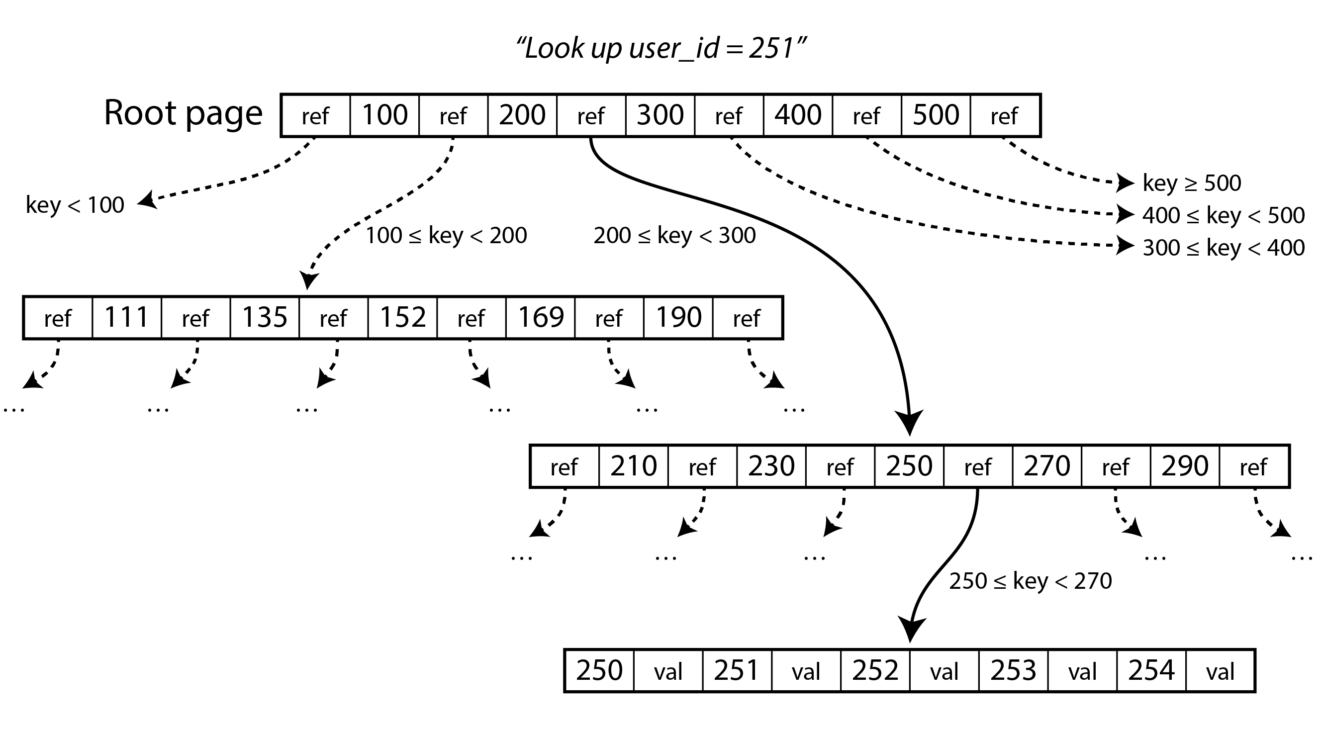
Figure 4-5 Looking up the key 251 using a B-tree index. From the root page we first follow the reference to the page for keys 200–300, then the page for keys 250–270.

One page is designated as the root of the B-tree; whenever you want to look up a key in the index, you start here. The page contains several keys and references to child pages. Each child is responsible for a continuous range of keys, and the keys between the references indicate where the boundaries between those ranges lie. (This structure is sometimes called a B+ tree, but we don’t need to distinguish it from other B-tree variants.)

In the example in Figure 4-5, we are looking for the key 251, so we know that we need to follow the page reference between the boundaries 200 and 300. That takes us to a similar-looking page that further breaks down the 200–300 range into subranges. Eventually we get down to a page containing individual keys (a leaf page), which either contains the value for each key inline or contains references to the pages where the values can be found.

The number of references to child pages in one page of the B-tree is called the branching factor. For example, in Figure 4-5 the branching factor is six. In practice, the branching factor depends on the amount of space required to store the page references and the range boundaries, but typically it is several hundred.

If you want to update the value for an existing key in a B-tree, you search for the leaf page containing that key, and overwrite that page on disk with a version that contains the new value. If you want to add a new key, you need to find the page whose range encompasses the new key and add it to that page. If there isn’t enough free space in the page to accommodate the new key, the page is split into two half-full pages, and the parent page is updated to account for the new subdivision of key ranges.

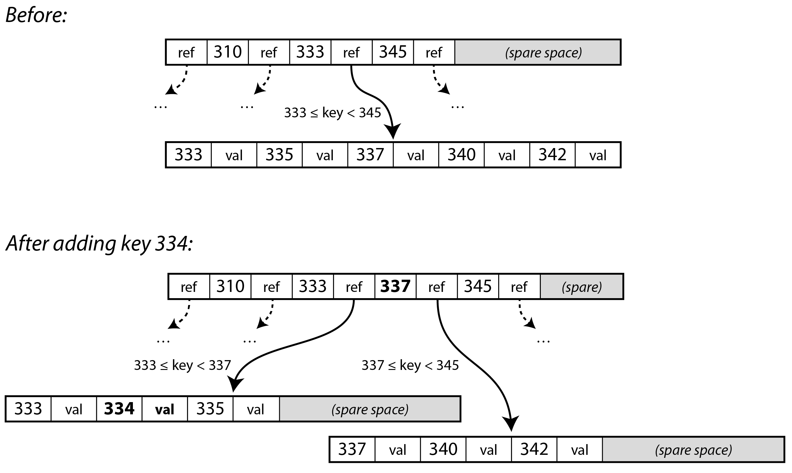
Figure 4-6 Growing a B-tree by splitting a page on the boundary key 337. The parent page is updated to reference both children.

In the example of Figure 4-6, we want to insert the key 334, but the page for the range 333–345 is already full. We therefore split it into a page for the range 333–337 (including the new key), and a page for 337–344. We also have to update the parent page to have references to both children, with a boundary value of 337 between them. If the parent page doesn’t have enough space for the new reference, it may also need to be split, and the splits can continue all the way to the root of the tree. When the root is split, we make a new root above it. Deleting keys (which may require nodes to be merged) is more complex ⁵.

This algorithm ensures that the tree remains balanced: a B-tree with n keys always has a depth of O(log n). Most databases can fit into a B-tree that is three or four levels deep, so you don’t need to follow many page references to find the page you are looking for. (A four-level tree of 4 KiB pages with a branching factor of 500 can store up to 250 TB.)

Making B-trees reliable

The basic underlying write operation of a B-tree is to overwrite a page on disk with new data. It is assumed that the overwrite does not change the location of the page; i.e., all references to that page remain intact when the page is overwritten. This is in stark contrast to log-structured indexes such as LSM-trees, which only append to files (and eventually delete obsolete files) but never modify files in place.

Overwriting several pages at once, like in a page split, is a dangerous operation: if the database crashes after only some of the pages have been written, you end up with a corrupted tree (e.g., there may be an orphan page that is not a child of any parent). If the hardware can’t atomically write an entire page, you can also end up with a partially written page (this is known as a torn page ²³).

In order to make the database resilient to crashes, it is common for B-tree implementations to include an additional data structure on disk: a write-ahead log (WAL). This is an append-only file to which every B-tree modification must be written before it can be applied to the pages of the tree itself. When the database comes back up after a crash, this log is used to restore the B-tree back to a consistent state ² ²⁴. In filesystems, the equivalent mechanism is known as journaling.

To improve performance, B-tree implementations typically don’t immediately write every modified page to disk, but buffer the B-tree pages in memory for a while first. The write-ahead log then also ensures that data is not lost in the case of a crash: as long as data has been written to the WAL, and flushed to disk using the fsync() system call, the data will be durable as the database will be able to recover it after a crash ²⁵.

B-tree variants

As B-trees have been around for so long, many variants have been developed over the years. To mention just a few:

Instead of overwriting pages and maintaining a WAL for crash recovery, some databases (like LMDB) use a copy-on-write scheme ²⁶. A modified page is written to a different location, and a new version of the parent pages in the tree is created, pointing at the new location. This approach is also useful for concurrency control, as we shall see in “Snapshot Isolation and Repeatable Read”.
We can save space in pages by not storing the entire key, but abbreviating it. Especially in pages on the interior of the tree, keys only need to provide enough information to act as boundaries between key ranges. Packing more keys into a page allows the tree to have a higher branching factor, and thus fewer levels.
To speed up scans over the key range in sorted order, some B-tree implementations try to lay out the tree so that leaf pages appear in sequential order on disk, reducing the number of disk seeks. However, it’s difficult to maintain that order as the tree grows.
Additional pointers have been added to the tree. For example, each leaf page may have references to its sibling pages to the left and right, which allows scanning keys in order without jumping back to parent pages.

Comparing B-Trees and LSM-Trees

As a rule of thumb, LSM-trees are better suited for write-heavy applications, whereas B-trees are faster for reads ²⁷ ²⁸. However, benchmarks are often sensitive to details of the workload. You need to test systems with your particular workload in order to make a valid comparison. Moreover, it’s not a strict either/or choice between LSM and B-trees: storage engines sometimes blend characteristics of both approaches, for example by having multiple B-trees and merging them LSM-style. In this section we will briefly discuss a few things that are worth considering when measuring the performance of a storage engine.

Read performance

In a B-tree, looking up a key involves reading one page at each level of the B-tree. Since the number of levels is usually quite small, this means that reads from a B-tree are generally fast and have predictable performance. In an LSM storage engine, reads often have to check several different SSTables at different stages of compaction, but Bloom filters help reduce the number of actual disk I/O operations required. Both approaches can perform well, and which is faster depends on the details of the storage engine and the workload.

Range queries are simple and fast on B-trees, as they can use the sorted structure of the tree. On LSM storage, range queries can also take advantage of the SSTable sorting, but they need to scan all the segments in parallel and combine the results. Bloom filters don’t help for range queries (since you would need to compute the hash of every possible key within the range, which is impractical), making range queries more expensive than point queries in the LSM approach ²⁹.

High write throughput can cause latency spikes in a log-structured storage engine if the memtable fills up. This happens if data can’t be written out to disk fast enough, perhaps because the compaction process cannot keep up with incoming writes. Many storage engines, including RocksDB, perform backpressure in this situation: they suspend all reads and writes until the memtable has been written out to disk ³⁰ ³¹.

Regarding read throughput, modern SSDs (and especially NVMe) can perform many independent read requests in parallel. Both LSM-trees and B-trees are able to provide high read throughput, but storage engines need to be carefully designed to take advantage of this parallelism ³².

Sequential vs. random writes

With a B-tree, if the application writes keys that are scattered all over the key space, the resulting disk operations are also scattered randomly, since the pages that the storage engine needs to overwrite could be located anywhere on disk. On the other hand, a log-structured storage engine writes entire segment files at a time (either writing out the memtable or while compacting existing segments), which are much bigger than a page in a B-tree.

The pattern of many small, scattered writes (as found in B-trees) is called random writes, while the pattern of fewer large writes (as found in LSM-trees) is called sequential writes. Disks generally have higher sequential write throughput than random write throughput, which means that a log-structured storage engine can generally handle higher write throughput on the same hardware than a B-tree. This difference is particularly big on spinning-disk hard drives (HDDs); on the solid state drives (SSDs) that most databases use today, the difference is smaller, but still noticeable (see “Sequential vs. Random Writes on SSDs”).

SEQUENTIAL VS. RANDOM WRITES ON SSDS

On spinning-disk hard drives (HDDs), sequential writes are much faster than random writes: a random write has to mechanically move the disk head to a new position and wait for the right part of the platter to pass underneath the disk head, which takes several milliseconds—an eternity in computing timescales. However, SSDs (solid-state drives) including NVMe (Non-Volatile Memory Express, i.e. flash memory attached to the PCI Express bus) have now overtaken HDDs for many use cases, and they are not subject to such mechanical limitations.

Nevertheless, SSDs also have higher throughput for sequential writes than for than random writes. The reason is that flash memory can be read or written one page (typically 4 KiB) at a time, but it can only be erased one block (typically 512 KiB) at a time. Some of the pages in a block may contain valid data, whereas others may contain data that is no longer needed. Before erasing a block, the controller must first move pages containing valid data into other blocks; this process is called garbage collection (GC) ³³.

A sequential write workload writes larger chunks of data at a time, so it is likely that a whole 512 KiB block belongs to a single file; when that file is later deleted again, the whole block can be erased without having to perform any GC. On the other hand, with a random write workload, it is more likely that a block contains a mixture of pages with valid and invalid data, so the GC has to perform more work before a block can be erased ³⁴ ³⁵ ³⁶.

The write bandwidth consumed by GC is then not available for the application. Moreover, the additional writes performed by GC contribute to wear on the flash memory; therefore, random writes wear out the drive faster than sequential writes.

Write amplification

With any type of storage engine, one write request from the application turns into multiple I/O operations on the underlying disk. With LSM-trees, a value is first written to the log for durability, then again when the memtable is written to disk, and again every time the key-value pair is part of a compaction. (If the values are significantly larger than the keys, this overhead can be reduced by storing values separately from keys, and performing compaction only on SSTables containing keys and references to values ³⁷.)

A B-tree index must write every piece of data at least twice: once to the write-ahead log, and once to the tree page itself. In addition, they sometimes need to write out an entire page, even if only a few bytes in that page changed, to ensure the B-tree can be correctly recovered after a crash or power failure ³⁸ ³⁹.

If you take the total number of bytes written to disk in some workload, and divide by the number of bytes you would have to write if you simply wrote an append-only log with no index, you get the write amplification. (Sometimes write amplification is defined in terms of I/O operations rather than bytes.) In write-heavy applications, the bottleneck might be the rate at which the database can write to disk. In this case, the higher the write amplification, the fewer writes per second it can handle within the available disk bandwidth.

Write amplification is a problem in both LSM-trees and B-trees. Which one is better depends on various factors, such as the length of your keys and values, and how often you overwrite existing keys versus insert new ones. For typical workloads, LSM-trees tend to have lower write amplification because they don’t have to write entire pages and they can compress chunks of the SSTable ⁴⁰. This is another factor that makes LSM storage engines well suited for write-heavy workloads.

Besides affecting throughput, write amplification is also relevant for the wear on SSDs: a storage engine with lower write amplification will wear out the SSD less quickly.

When measuring the write throughput of a storage engine, it is important to run the experiment for long enough that the effects of write amplification become clear. When writing to an empty LSM-tree, there are no compactions going on yet, so all of the disk bandwidth is available for new writes. As the database grows, new writes need to share the disk bandwidth with compaction.

Disk space usage

B-trees can become fragmented over time: for example, if a large number of keys are deleted, the database file may contain a lot of pages that are no longer used by the B-tree. Subsequent additions to the B-tree can use those free pages, but they can’t easily be returned to the operating system because they are in the middle of the file, so they still take up space on the filesystem. Databases therefore need a background process that moves pages around to place them better, such as the vacuum process in PostgreSQL ²⁵.

Fragmentation is less of a problem in LSM-trees, since the compaction process periodically rewrites the data files anyway, and SSTables don’t have pages with unused space. Moreover, blocks of key-value pairs can better be compressed in SSTables, and thus often produce smaller files on disk than B-trees. Keys and values that have been overwritten continue to consume space until they are removed by a compaction, but this overhead is quite low when using leveled compaction ⁴⁰ ⁴¹. Size-tiered compaction (see “Compaction strategies”) uses more disk space, especially temporarily during compaction.

Having multiple copies of some data on disk can also be a problem when you need to delete some data, and be confident that it really has been deleted (perhaps to comply with data protection regulations). For example, in most LSM storage engines a deleted record may still exist in the higher levels until the tombstone representing the deletion has been propagated through all of the compaction levels, which may take a long time. Specialist storage engine designs can propagate deletions faster ⁴².

On the other hand, the immutable nature of SSTable segment files is useful if you want to take a snapshot of a database at some point in time (e.g. for a backup or to create a copy of the database for testing): you can write out the memtable and record which segment files existed at that point in time. As long as you don’t delete the files that are part of the snapshot, you don’t need to actually copy them. In a B-tree whose pages are overwritten, taking such a snapshot efficiently is more difficult.

Multi-Column and Secondary Indexes

So far we have only discussed key-value indexes, which are like a primary key index in the relational model. A primary key uniquely identifies one row in a relational table, or one document in a document database, or one vertex in a graph database. Other records in the database can refer to that row/document/vertex by its primary key (or ID), and the index is used to resolve such references.

It is also very common to have secondary indexes. In relational databases, you can create several secondary indexes on the same table using the CREATE INDEX command, allowing you to search by columns other than the primary key. For example, in Figure 3-1 in Chapter 3 you would most likely have a secondary index on the user_id columns so that you can find all the rows belonging to the same user in each of the tables.

A secondary index can easily be constructed from a key-value index. The main difference is that in a secondary index, the indexed values are not necessarily unique; that is, there might be many rows (documents, vertices) under the same index entry. This can be solved in two ways: either by making each value in the index a list of matching row identifiers (like a postings list in a full-text index) or by making each entry unique by appending a row identifier to it. Storage engines with in-place updates, like B-trees, and log-structured storage can both be used to implement an index.

Storing values within the index

The key in an index is the thing that queries search by, but the value can be one of several things:

If the actual data (row, document, vertex) is stored directly within the index structure, it is called a clustered index. For example, in MySQL’s InnoDB storage engine, the primary key of a table is always a clustered index, and in SQL Server, you can specify one clustered index per table ⁴³.
Alternatively, the value can be a reference to the actual data: either the primary key of the row in question (InnoDB does this for secondary indexes), or a direct reference to a location on disk. In the latter case, the place where rows are stored is known as a heap file, and it stores data in no particular order (it may be append-only, or it may keep track of deleted rows in order to overwrite them with new data later). For example, Postgres uses the heap file approach ⁴⁴.
A middle ground between the two is a covering index or index with included columns, which stores some of a table’s columns within the index, in addition to storing the full row on the heap or in the primary key clustered index ⁴⁵. This allows some queries to be answered by using the index alone, without having to resolve the primary key or look in the heap file (in which case, the index is said to cover the query). This can make some queries faster, but the duplication of data means the index uses more disk space and slows down writes.

The indexes discussed so far only map a single key to a value. If you need to query multiple columns of a table (or multiple fields in a document) simultaneously, see “Multidimensional and Full-Text Indexes”.

When updating a value without changing the key, the heap file approach can allow the record to be overwritten in place, provided that the new value is not larger than the old value. The situation is more complicated if the new value is larger, as it probably needs to be moved to a new location in the heap where there is enough space. In that case, either all indexes need to be updated to point at the new heap location of the record, or a forwarding pointer is left behind in the old heap location ².

Keeping everything in memory

The data structures discussed so far in this chapter have all been answers to the limitations of disks. Compared to main memory, disks are awkward to deal with. With both magnetic disks and SSDs, data on disk needs to be laid out carefully if you want good performance on reads and writes. However, we tolerate this awkwardness because disks have two significant advantages: they are durable (their contents are not lost if the power is turned off), and they have a lower cost per gigabyte than RAM.

As RAM becomes cheaper, the cost-per-gigabyte argument is eroded. Many datasets are simply not that big, so it’s quite feasible to keep them entirely in memory, potentially distributed across several machines. This has led to the development of in-memory databases.

Some in-memory key-value stores, such as Memcached, are intended for caching use only, where it’s acceptable for data to be lost if a machine is restarted. But other in-memory databases aim for durability, which can be achieved with special hardware (such as battery-powered RAM), by writing a log of changes to disk, by writing periodic snapshots to disk, or by replicating the in-memory state to other machines.

When an in-memory database is restarted, it needs to reload its state, either from disk or over the network from a replica (unless special hardware is used). Despite writing to disk, it’s still an in-memory database, because the disk is merely used as an append-only log for durability, and reads are served entirely from memory. Writing to disk also has operational advantages: files on disk can easily be backed up, inspected, and analyzed by external utilities.

Products such as VoltDB, SingleStore, and Oracle TimesTen are in-memory databases with a relational model, and the vendors claim that they can offer big performance improvements by removing all the overheads associated with managing on-disk data structures ⁴⁶ ⁴⁷. RAMCloud is an open source, in-memory key-value store with durability (using a log-structured approach for the data in memory as well as the data on disk) ⁴⁸.

Redis and Couchbase provide weak durability by writing to disk asynchronously.

Counterintuitively, the performance advantage of in-memory databases is not due to the fact that they don’t need to read from disk. Even a disk-based storage engine may never need to read from disk if you have enough memory, because the operating system caches recently used disk blocks in memory anyway. Rather, they can be faster because they can avoid the overheads of encoding in-memory data structures in a form that can be written to disk ⁴⁹.

Besides performance, another interesting area for in-memory databases is providing data models that are difficult to implement with disk-based indexes. For example, Redis offers a database-like interface to various data structures such as priority queues and sets. Because it keeps all data in memory, its implementation is comparatively simple.

Data Storage for Analytics

The data model of a data warehouse is most commonly relational, because SQL is generally a good fit for analytic queries. There are many graphical data analysis tools that generate SQL queries, visualize the results, and allow analysts to explore the data (through operations such as drill-down and slicing and dicing).

On the surface, a data warehouse and a relational OLTP database look similar, because they both have a SQL query interface. However, the internals of the systems can look quite different, because they are optimized for very different query patterns. Many database vendors now focus on supporting either transaction processing or analytics workloads, but not both.

Some databases, such as Microsoft SQL Server, SAP HANA, and SingleStore, have support for transaction processing and data warehousing in the same product. However, these hybrid transactional and analytical processing (HTAP) databases (introduced in “Data Warehousing”) are increasingly becoming two separate storage and query engines, which happen to be accessible through a common SQL interface ⁵⁰ ⁵¹ ⁵² ⁵³.

Cloud Data Warehouses

Data warehouse vendors such as Teradata, Vertica, and SAP HANA sell both on-premises warehouses under commercial licenses and cloud-based solutions. But as many of their customers move to the cloud, new cloud data warehouses such as Google Cloud BigQuery, Amazon Redshift, and Snowflake have also become widely adopted. Unlike traditional data warehouses, cloud data warehouses take advantage of scalable cloud infrastructure like object storage and serverless computation platforms.

Cloud data warehouses tend to integrate better with other cloud services and to be more elastic. For example, many cloud warehouses support automatic log ingestion, and offer easy integration with data processing frameworks such as Google Cloud’s Dataflow or Amazon Web Services’ Kinesis. These warehouses are also more elastic because they decouple query computation from the storage layer ⁵⁴. Data is persisted on object storage rather than local disks, which makes it easy to adjust storage capacity and compute resources for queries independently, as we previously saw in “Cloud-Native System Architecture”.

Open source data warehouses such as Apache Hive, Trino, and Apache Spark have also evolved with the cloud. As data storage for analytics has moved to data lakes on object storage, open source warehouses have begun to break apart ⁵⁵. The following components, which were previously integrated in a single system such as Apache Hive, are now often implemented as separate components:

Query engine: Query engines such as Trino, Apache DataFusion, and Presto parse SQL queries, optimize them into execution plans, and execute them against the data. Execution usually requires parallel, distributed data processing tasks. Some query engines provide built-in task execution, while others choose to use third party execution frameworks such as Apache Spark or Apache Flink.
Storage format: The storage format determines how the rows of a table are encoded as bytes in a file, which is then typically stored in object storage or a distributed filesystem ¹². This data can then be accessed by the query engine, but also by other applications using the data lake. Examples of such storage formats are Parquet, ORC, Lance, or Nimble, and we will see more about them in the next section.
Table format: Files written in Apache Parquet and similar storage formats are typically immutable once written. To support row inserts and deletions, a table format such as Apache Iceberg or Databricks’s Delta format are used. Table formats specify a file format that defines which files constitute a table along with the table’s schema. Such formats also offer advanced features such as time travel (the ability to query a table as it was at a previous point in time), garbage collection, and even transactions.
Data catalog: Much like a table format defines which files make up a table, a data catalog defines which tables comprise a database. Catalogs are used to create, rename, and drop tables. Unlike storage and table formats, data catalogs such as Snowflake’s Polaris and Databricks’s Unity Catalog usually run as a standalone service that can be queried using a REST interface. Apache Iceberg also offers a catalog, which can be run inside a client or as a separate process. Query engines use catalog information when reading and writing tables. Traditionally, catalogs and query engines have been integrated, but decoupling them has enabled data discovery and data governance systems (discussed in “Data Systems, Law, and Society”) to access a catalog’s metadata as well.

Column-Oriented Storage

As discussed in “Stars and Snowflakes: Schemas for Analytics”, data warehouses by convention often use a relational schema with a big fact table that contains foreign key references into dimension tables. If you have trillions of rows and petabytes of data in your fact tables, storing and querying them efficiently becomes a challenging problem. Dimension tables are usually much smaller (millions of rows), so in this section we will focus on storage of facts.

Although fact tables are often over 100 columns wide, a typical data warehouse query only accesses 4 or 5 of them at one time ("SELECT *" queries are rarely needed for analytics) ⁵². Take the query in Example 4-1: it accesses a large number of rows (every occurrence of someone buying fruit or candy during the 2024 calendar year), but it only needs to access three columns of the fact_sales table: date_key, product_sk, and quantity. The query ignores all other columns.

Example 4-1. Analyzing whether people are more inclined to buy fresh fruit or candy, depending on the day of the week

SELECT
    dim_date.weekday, dim_product.category,
    SUM(fact_sales.quantity) AS quantity_sold
FROM fact_sales
    JOIN dim_date ON fact_sales.date_key = dim_date.date_key
    JOIN dim_product ON fact_sales.product_sk = dim_product.product_sk
WHERE
    dim_date.year = 2024 AND
    dim_product.category IN ('Fresh fruit', 'Candy')
GROUP BY
    dim_date.weekday, dim_product.category;

How can we execute this query efficiently?

In most OLTP databases, storage is laid out in a row-oriented fashion: all the values from one row of a table are stored next to each other. Document databases are similar: an entire document is typically stored as one contiguous sequence of bytes. You can see this in the CSV example of Figure 4-1.

In order to process a query like Example 4-1, you may have indexes on fact_sales.date_key and/or fact_sales.product_sk that tell the storage engine where to find all the sales for a particular date or for a particular product. But then, a row-oriented storage engine still needs to load all of those rows (each consisting of over 100 attributes) from disk into memory, parse them, and filter out those that don’t meet the required conditions. That can take a long time.

The idea behind column-oriented (or columnar) storage is simple: don’t store all the values from one row together, but store all the values from each column together instead ⁵⁶. If each column is stored separately, a query only needs to read and parse those columns that are used in that query, which can save a lot of work. Figure 4-7 shows this principle using an expanded version of the fact table from Figure 3-5.

Note

Column storage is easiest to understand in a relational data model, but it applies equally to nonrelational data. For example, Parquet ⁵⁷ is a columnar storage format that supports a document data model, based on Google’s Dremel ⁵⁸, using a technique known as shredding or striping ⁵⁹.

Figure 4-7 Storing relational data by column, rather than by row.

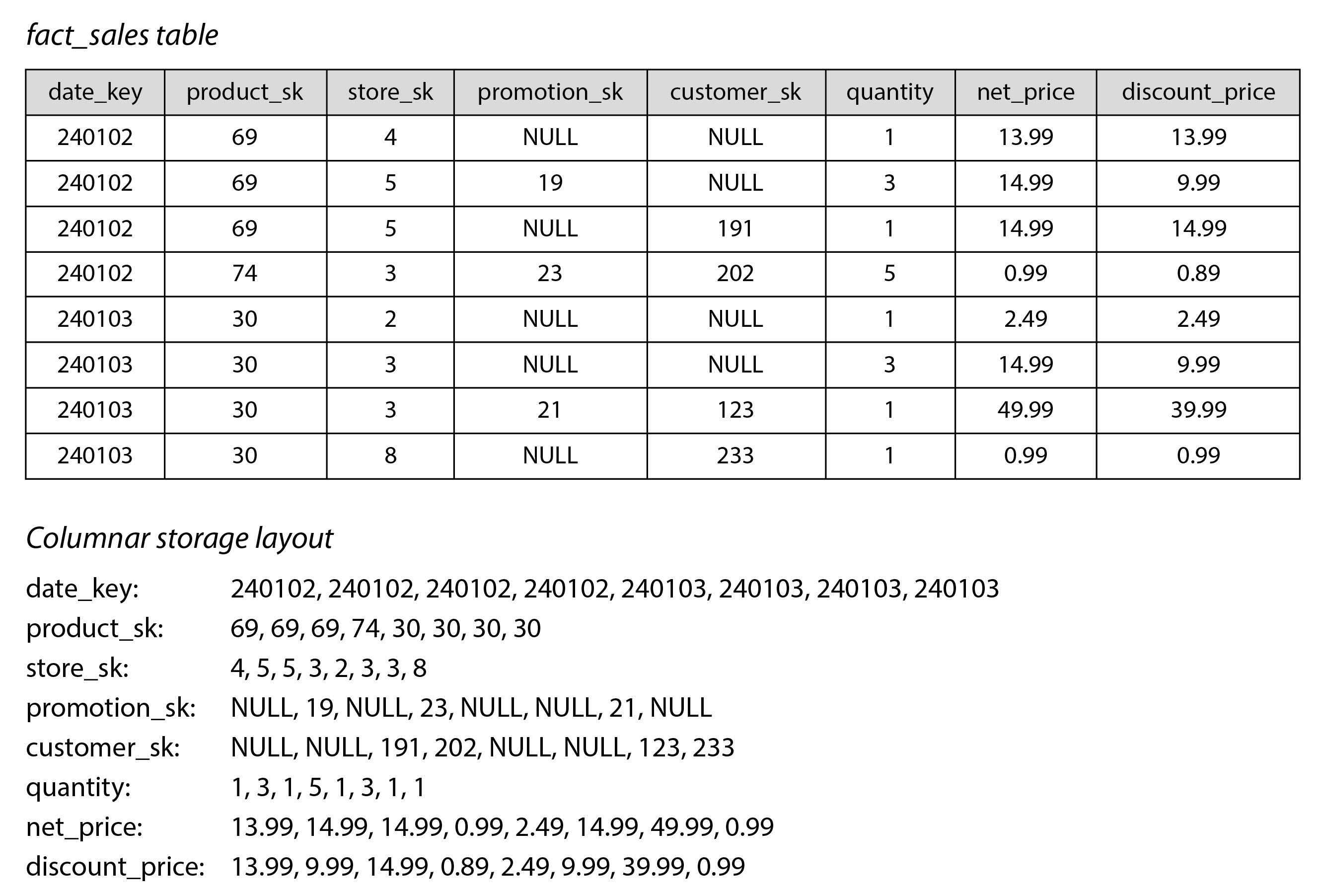
The column-oriented storage layout relies on each column storing the rows in the same order. Thus, if you need to reassemble an entire row, you can take the 23rd entry from each of the individual columns and put them together to form the 23rd row of the table.

In fact, columnar storage engines don’t actually store an entire column (containing perhaps trillions of rows) in one go. Instead, they break the table into blocks of thousands or millions of rows, and within each block they store the values from each column separately ⁶⁰. Since many queries are restricted to a particular date range, it is common to make each block contain the rows for a particular timestamp range. A query then only needs to load the columns it needs in those blocks that overlap with the required date range.

Columnar storage is used in almost all analytic databases nowadays ⁶⁰, ranging from large-scale cloud data warehouses such as Snowflake ⁶¹ to single-node embedded databases such as DuckDB ⁶², and product analytics systems such as Pinot ⁶³ and Druid ⁶⁴. It is used in storage formats such as Parquet, ORC ⁶⁵ ⁶⁶, Lance ⁶⁷, and Nimble ⁶⁸, and in-memory analytics formats like Apache Arrow ⁶⁵ ⁶⁹ and Pandas/NumPy ⁷⁰. Some time-series databases, such as InfluxDB IOx ⁷¹ and TimescaleDB ⁷², are also based on column-oriented storage.

Column Compression

Besides only loading those columns from disk that are required for a query, we can further reduce the demands on disk throughput and network bandwidth by compressing data. Fortunately, column-oriented storage often lends itself very well to compression.

Take a look at the sequences of values for each column in Figure 4-7: they often look quite repetitive, which is a good sign for compression. Depending on the data in the column, different compression techniques can be used. One technique that is particularly effective in data warehouses is bitmap encoding, illustrated in Figure 4-8.

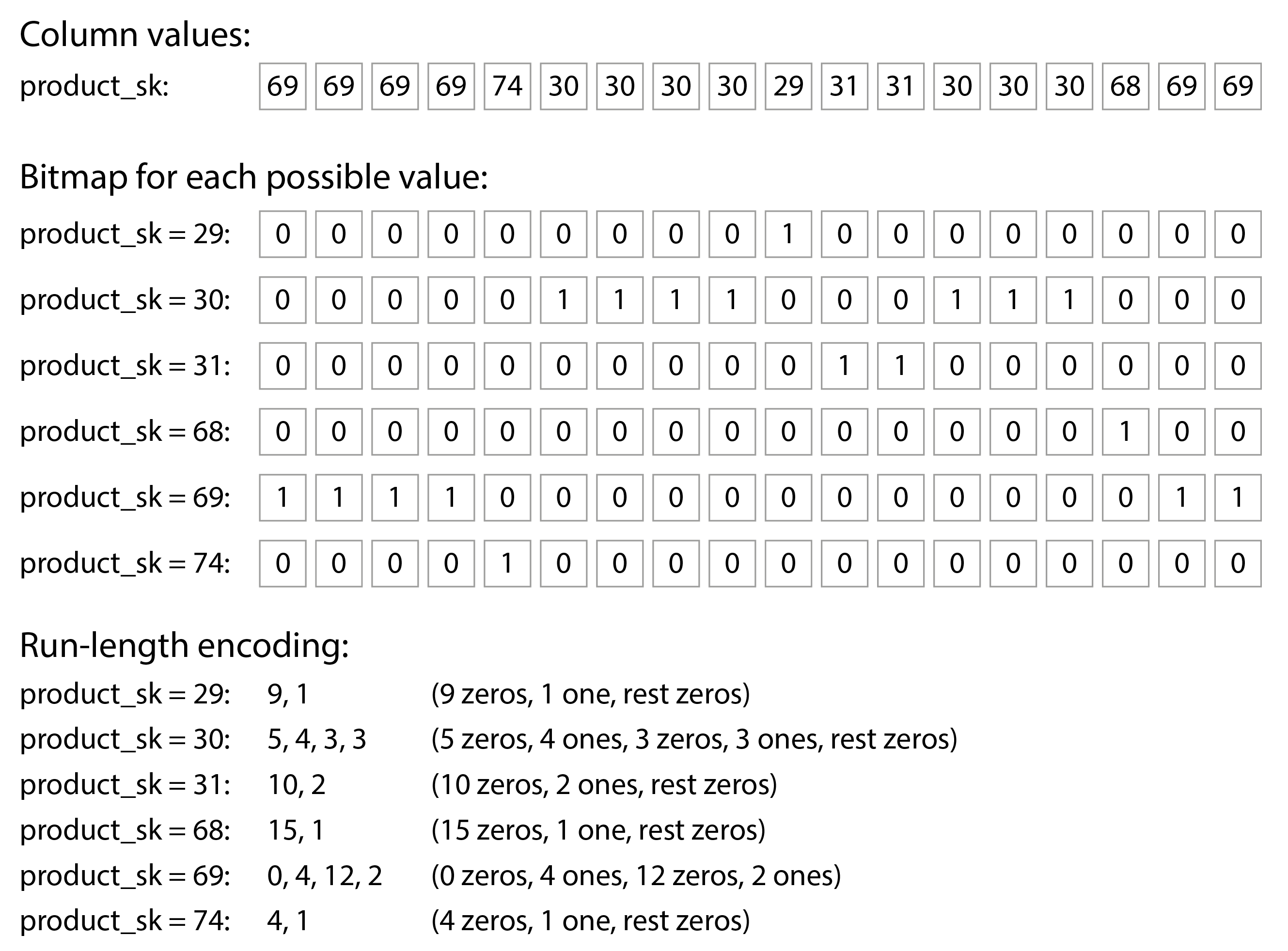
Figure 4-8 Compressed, bitmap-indexed storage of a single column.

Often, the number of distinct values in a column is small compared to the number of rows (for example, a retailer may have billions of sales transactions, but only 100,000 distinct products). We can now take a column with n distinct values and turn it into n separate bitmaps: one bitmap for each distinct value, with one bit for each row. The bit is 1 if the row has that value, and 0 if not.

One option is to store those bitmaps using one bit per row. However, these bitmaps typically contain a lot of zeros (we say that they are sparse). In that case, the bitmaps can additionally be run-length encoded: counting the number of consecutive zeros or ones and storing that number, as shown at the bottom of Figure 4-8. Techniques such as roaring bitmaps switch between the two bitmap representations, using whichever is the most compact ⁷³. This can make the encoding of a column remarkably efficient.

Bitmap indexes such as these are very well suited for the kinds of queries that are common in a data warehouse. For example:

WHERE product_sk IN (31, 68, 69):: Load the three bitmaps for product_sk = 31, product_sk = 68, and product_sk = 69, and calculate the bitwise OR of the three bitmaps, which can be done very efficiently.
WHERE product_sk = 30 AND store_sk = 3:: Load the bitmaps for product_sk = 30 and store_sk = 3, and calculate the bitwise AND. This works because the columns contain the rows in the same order, so the kth bit in one column’s bitmap corresponds to the same row as the kth bit in another column’s bitmap.

Bitmaps can also be used to answer graph queries, such as finding all users of a social network who are followed by user X and who also follow user Y ⁷⁴. There are also various other compression schemes for columnar databases, which you can find in the references ⁷⁵.

Note

Don’t confuse column-oriented databases with the wide-column (also known as column-family) data model, in which a row can have thousands of columns, and there is no need for all the rows to have the same columns ⁹. Despite the similarity in name, wide-column databases are row-oriented, since they store all values from a row together. Google’s Bigtable, Apache Accumulo, and HBase are examples of the wide-column model.

Sort Order in Column Storage

In a column store, it doesn’t necessarily matter in which order the rows are stored. It’s easiest to store them in the order in which they were inserted, since then inserting a new row just means appending to each of the columns. However, we can choose to impose an order, like we did with SSTables previously, and use that as an indexing mechanism.

Note that it wouldn’t make sense to sort each column independently, because then we would no longer know which items in the columns belong to the same row. We can only reconstruct a row because we know that the kth item in one column belongs to the same row as the kth item in another column.

Rather, the data needs to be sorted an entire row at a time, even though it is stored by column. The administrator of the database can choose the columns by which the table should be sorted, using their knowledge of common queries. For example, if queries often target date ranges, such as the last month, it might make sense to make date_key the first sort key. Then the query can scan only the rows from the last month, which will be much faster than scanning all rows.

A second column can determine the sort order of any rows that have the same value in the first column. For example, if date_key is the first sort key in Figure 4-7, it might make sense for product_sk to be the second sort key so that all sales for the same product on the same day are grouped together in storage. That will help queries that need to group or filter sales by product within a certain date range.

Another advantage of sorted order is that it can help with compression of columns. If the primary sort column does not have many distinct values, then after sorting, it will have long sequences where the same value is repeated many times in a row. A simple run-length encoding, like we used for the bitmaps in Figure 4-8, could compress that column down to a few kilobytes—even if the table has billions of rows.

That compression effect is strongest on the first sort key. The second and third sort keys will be more jumbled up, and thus not have such long runs of repeated values. Columns further down the sorting priority appear in essentially random order, so they probably won’t compress as well. But having the first few columns sorted is still a win overall.

Writing to Column-Oriented Storage

We saw in “Characterizing Transaction Processing and Analytics” that reads in data warehouses tend to consist of aggregations over a large number of rows; column-oriented storage, compression, and sorting all help to make those read queries faster. Writes in a data warehouse tend to be a bulk import of data, often via an ETL process.

With columnar storage, writing an individual row somewhere in the middle of a sorted table would be very inefficient, as you would have to rewrite all the compressed columns from the insertion position onwards. However, a bulk write of many rows at once amortizes the cost of rewriting those columns, making it efficient.

A log-structured approach is often used to perform writes in batches. All writes first go to a row-oriented, sorted, in-memory store. When enough writes have accumulated, they are merged with the column-encoded files on disk and written to new files in bulk. As old files remain immutable, and new files are written in one go, object storage is well suited for storing these files.

Queries need to examine both the column data on disk and the recent writes in memory, and combine the two. The query execution engine hides this distinction from the user. From an analyst’s point of view, data that has been modified with inserts, updates, or deletes is immediately reflected in subsequent queries. Snowflake, Vertica, Apache Pinot, Apache Druid, and many others do this ⁶¹ ⁶³ ⁶⁴ ⁷⁶.

Query Execution: Compilation and Vectorization

A complex SQL query for analytics is broken down into a query plan consisting of multiple stages, called operators, which may be distributed across multiple machines for parallel execution. Query planners can perform a lot of optimizations by choosing which operators to use, in which order to perform them, and where to run each operator.

Within each operator, the query engine needs to do various things with the values in a column, such as finding all the rows where the value is among a particular set of values (perhaps as part of a join), or checking whether the value is greater than 15. It also needs to look at several columns for the same row, for example to find all sales transactions where the product is bananas and the store is a particular store of interest.

For data warehouse queries that need to scan over millions of rows, we need to worry not only about the amount of data they need to read off disk, but also the CPU time required to execute complex operators. The simplest kind of operator is like an interpreter for a programming language: while iterating over each row, it checks a data structure representing the query to find out which comparisons or calculations it needs to perform on which columns. Unfortunately, this is too slow for many analytics purposes. Two alternative approaches for efficient query execution have emerged ⁷⁷:

Query compilation: The query engine takes the SQL query and generates code for executing it. The code iterates over the rows one by one, looks at the values in the columns of interest, performs whatever comparisons or calculations are needed, and copies the necessary values to an output buffer if the required conditions are satisfied. The query engine compiles the generated code to machine code (often using an existing compiler such as LLVM), and then runs it on the column-encoded data that has been loaded into memory. This approach to code generation is similar to the just-in-time (JIT) compilation approach that is used in the Java Virtual Machine (JVM) and similar runtimes.
Vectorized processing: The query is interpreted, not compiled, but it is made fast by processing many values from a column in a batch, instead of iterating over rows one by one. A fixed set of predefined operators are built into the database; we can pass arguments to them and get back a batch of results ⁵⁰ ⁷⁵.

For example, we could pass the product_sk column and the ID of “bananas” to an equality operator, and get back a bitmap (one bit per value in the input column, which is 1 if it’s a banana); we could then pass the store_sk column and the ID of the store of interest to the same equality operator, and get back another bitmap; and then we could pass the two bitmaps to a “bitwise AND” operator, as shown in Figure 4-9. The result would be a bitmap containing a 1 for all sales of bananas in a particular store.

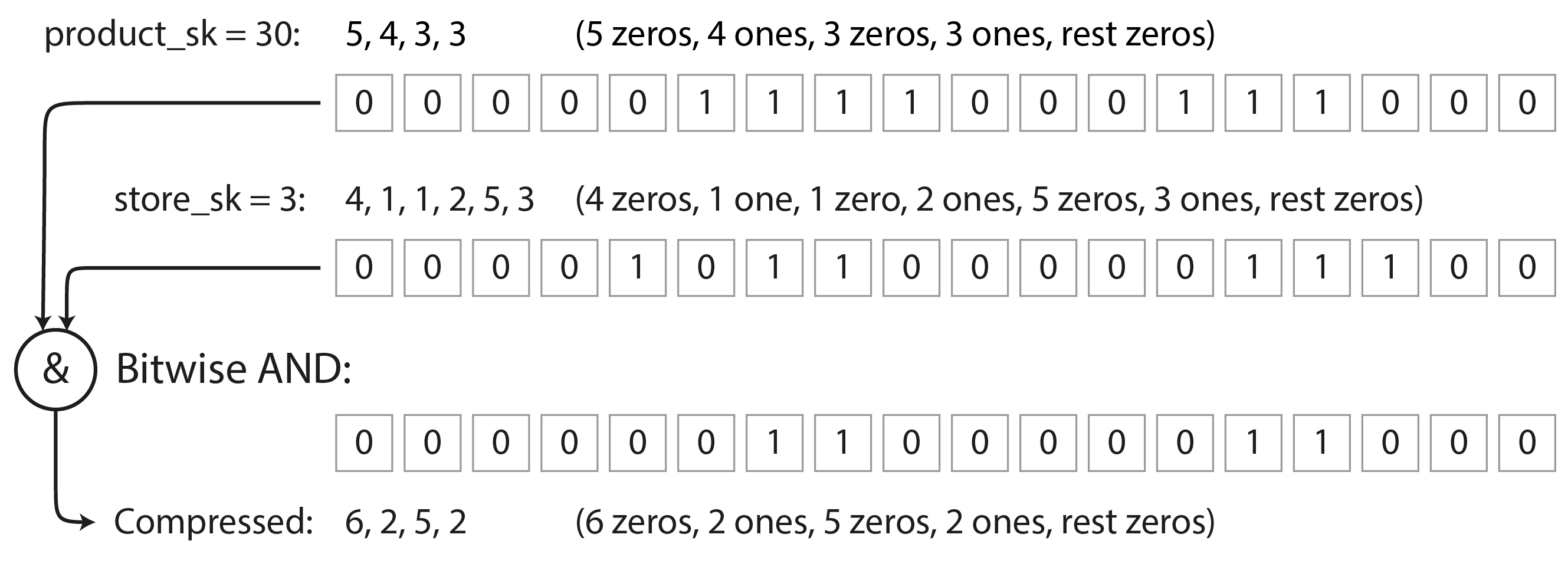
Figure 4-9 A bitwise AND between two bitmaps lends itself to vectorization.

The two approaches are very different in terms of their implementation, but both are used in practice ⁷⁷. Both can achieve very good performance by taking advantages of the characteristics of modern CPUs:

preferring sequential memory access over random access to reduce cache misses ⁷⁸,
doing most of the work in tight inner loops (that is, with a small number of instructions and no function calls) to keep the CPU instruction processing pipeline busy and avoid branch mispredictions,
making use of parallelism such as multiple threads and single-instruction-multi-data (SIMD) instructions ⁷⁹ ⁸⁰, and
operating directly on compressed data without decoding it into a separate in-memory representation, which saves memory allocation and copying costs.

Materialized Views and Data Cubes

We previously encountered materialized views in “Materializing and Updating Timelines”: in a relational data model, they are table-like object whose contents are the results of some query. The difference is that a materialized view is an actual copy of the query results, written to disk, whereas a virtual view is just a shortcut for writing queries. When you read from a virtual view, the SQL engine expands it into the view’s underlying query on the fly and then processes the expanded query.

When the underlying data changes, a materialized view needs to be updated accordingly. Some databases can do that automatically, and there are also systems such as Materialize that specialize in materialized view maintenance ⁸¹. Performing such updates means more work on writes, but materialized views can improve read performance in workloads that repeatedly need to perform the same queries.

Materialized aggregates are a type of materialized views that can be useful in data warehouses. As discussed earlier, data warehouse queries often involve an aggregate function, such as COUNT, SUM, AVG, MIN, or MAX in SQL. If the same aggregates are used by many different queries, it can be wasteful to crunch through the raw data every time. Why not cache some of the counts or sums that queries use most often? A data cube or OLAP cube does this by creating a grid of aggregates grouped by different dimensions ⁸². Figure 4-10 shows an example.

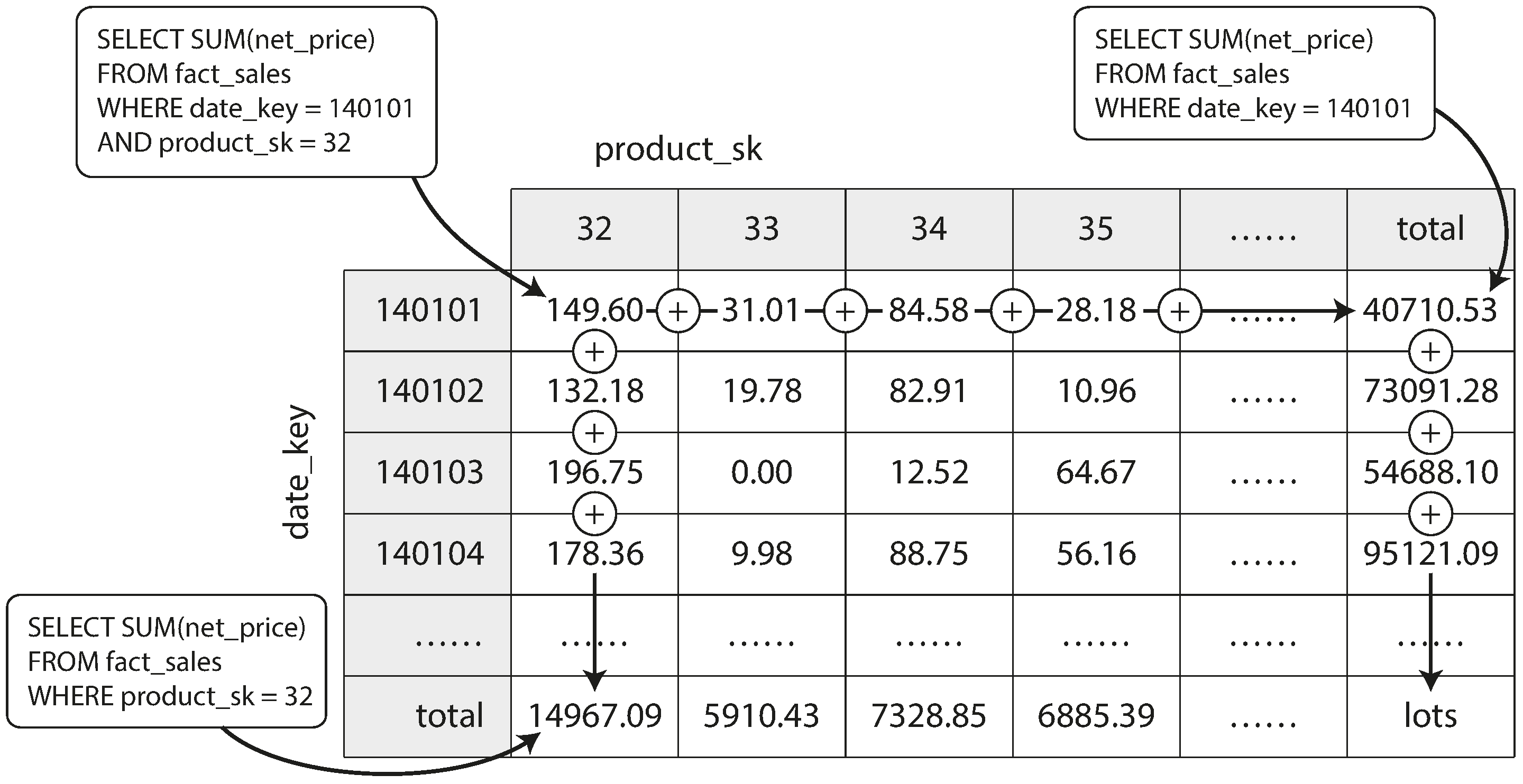
Figure 4-10 Two dimensions of a data cube, aggregating data by summing.

Imagine for now that each fact has foreign keys to only two dimension tables—in Figure 4-10, these are date_key and product_sk. You can now draw a two-dimensional table, with dates along one axis and products along the other. Each cell contains the aggregate (e.g., SUM) of an attribute (e.g., net_price) of all facts with that date-product combination. Then you can apply the same aggregate along each row or column and get a summary that has been reduced by one dimension (the sales by product regardless of date, or the sales by date regardless of product).

In general, facts often have more than two dimensions. In Figure 3-5 there are five dimensions: date, product, store, promotion, and customer. It’s a lot harder to imagine what a five-dimensional hypercube would look like, but the principle remains the same: each cell contains the sales for a particular date-product-store-promotion-customer combination. These values can then repeatedly be summarized along each of the dimensions.

The advantage of a materialized data cube is that certain queries become very fast because they have effectively been precomputed. For example, if you want to know the total sales per store yesterday, you just need to look at the totals along the appropriate dimension—no need to scan millions of rows.

The disadvantage is that a data cube doesn’t have the same flexibility as querying the raw data. For example, there is no way of calculating which proportion of sales comes from items that cost more than $100, because the price isn’t one of the dimensions. Most data warehouses therefore try to keep as much raw data as possible, and use aggregates such as data cubes only as a performance boost for certain queries.

Multidimensional and Full-Text Indexes

The B-trees and LSM-trees we saw in the first half of this chapter allow range queries over a single attribute: for example, if the key is a username, you can use them as an index to efficiently find all names starting with an L. But sometimes, searching by a single attribute is not enough.

The most common type of multi-column index is called a concatenated index, which simply combines several fields into one key by appending one column to another (the index definition specifies in which order the fields are concatenated). This is like an old-fashioned paper phone book, which provides an index from (lastname, firstname) to phone number. Due to the sort order, the index can be used to find all the people with a particular last name, or all the people with a particular lastname-firstname combination. However, the index is useless if you want to find all the people with a particular first name.

On the other hand, multi-dimensional indexes allow you to query several columns at once. One case where this is particularly important is geospatial data. For example, a restaurant-search website may have a database containing the latitude and longitude of each restaurant. When a user is looking at the restaurants on a map, the website needs to search for all the restaurants within the rectangular map area that the user is currently viewing. This requires a two-dimensional range query like the following:

SELECT * FROM restaurants WHERE latitude > 51.4946 AND latitude < 51.5079
    AND longitude > -0.1162 AND longitude < -0.1004;

A concatenated index over the latitude and longitude columns is not able to answer that kind of query efficiently: it can give you either all the restaurants in a range of latitudes (but at any longitude), or all the restaurants in a range of longitudes (but anywhere between the North and South poles), but not both simultaneously.

One option is to translate a two-dimensional location into a single number using a space-filling curve, and then to use a regular B-tree index ⁸³. More commonly, specialized spatial indexes such as R-trees or Bkd-trees ⁸⁴ are used; they divide up the space so that nearby data points tend to be grouped in the same subtree. For example, PostGIS implements geospatial indexes as R-trees using PostgreSQL’s Generalized Search Tree indexing facility ⁸⁵. It is also possible to use regularly spaced grids of triangles, squares, or hexagons ⁸⁶.

Multi-dimensional indexes are not just for geographic locations. For example, on an ecommerce website you could use a three-dimensional index on the dimensions (red, green, blue) to search for products in a certain range of colors, or in a database of weather observations you could have a two-dimensional index on (date, temperature) in order to efficiently search for all the observations during the year 2013 where the temperature was between 25 and 30℃. With a one-dimensional index, you would have to either scan over all the records from 2013 (regardless of temperature) and then filter them by temperature, or vice versa. A 2D index could narrow down by timestamp and temperature simultaneously ⁸⁷.

Full-Text Search

Full-text search allows you to search a collection of text documents (web pages, product descriptions, etc.) by keywords that might appear anywhere in the text ⁸⁸. Information retrieval is a big, specialist topic that often involves language-specific processing: for example, several Asian languages are written without spaces or punctuation between words, and therefore splitting text into words requires a model that indicates which character sequences constitute a word. Full-text search also often involves matching words that are similar but not identical (such as typos or different grammatical forms of words) and synonyms. Those problems go beyond the scope of this book.

However, at its core, you can think of full-text search as another kind of multidimensional query: in this case, each word that might appear in a text (a term) is a dimension. A document that contains term x has a value of 1 in dimension x, and a document that doesn’t contain x has a value of 0. Searching for documents mentioning “red apples” means a query that looks for a 1 in the red dimension, and simultaneously a 1 in the apples dimension. The number of dimensions may thus be very large.

The data structure that many search engines use to answer such queries is called an inverted index. This is a key-value structure where the key is a term, and the value is the list of IDs of all the documents that contain the term (the postings list). If the document IDs are sequential numbers, the postings list can also be represented as a sparse bitmap, like in Figure 4-8: the nth bit in the bitmap for term x is a 1 if the document with ID n contains the term x ⁸⁹.

Finding all the documents that contain both terms x and y is now similar to a vectorized data warehouse query that searches for rows matching two conditions (Figure 4-9): load the two bitmaps for terms x and y and compute their bitwise AND. Even if the bitmaps are run-length encoded, this can be done very efficiently.

For example, Lucene, the full-text indexing engine used by Elasticsearch and Solr, works like this ⁹⁰. It stores the mapping from term to postings list in SSTable-like sorted files, which are merged in the background using the same log-structured approach we saw earlier in this chapter ⁹¹. PostgreSQL’s GIN index type also uses postings lists to support full-text search and indexing inside JSON documents ⁹² ⁹³.

Instead of breaking text into words, an alternative is to find all the substrings of length n, which are called n-grams. For example, the trigrams (n = 3) of the string "hello" are "hel", "ell", and "llo". If we build an inverted index of all trigrams, we can search the documents for arbitrary substrings that are at least three characters long. Trigram indexes even allows regular expressions in search queries; the downside is that they are quite large ⁹⁴.

To cope with typos in documents or queries, Lucene is able to search text for words within a certain edit distance (an edit distance of 1 means that one letter has been added, removed, or replaced) ⁹⁵. It does this by storing the set of terms as a finite state automaton over the characters in the keys, similar to a trie ⁹⁶, and transforming it into a Levenshtein automaton, which supports efficient search for words within a given edit distance ⁹⁷.

Vector Embeddings

Semantic search goes beyond synonyms and typos to try and understand document concepts and user intentions. For example, if your help pages contain a page titled “cancelling your subscription”, users should still be able to find that page when searching for “how to close my account” or “terminate contract”, which are close in terms of meaning even though they use completely different words.

To understand a document’s semantics—its meaning—semantic search indexes use embedding models to translate a document into a vector of floating-point values, called a vector embedding. The vector represents a point in a multi-dimensional space, and each floating-point value represents the document’s location along one dimension’s axis. Embedding models generate vector embeddings that are near each other (in this multi-dimensional space) when the embedding’s input documents are semantically similar.

Note

We saw the term vectorized processing in “Query Execution: Compilation and Vectorization”. Vectors in semantic search have a different meaning. In vectorized processing, the vector refers to a batch of bits that can be processed with specially optimized code. In embedding models, vectors are a list of floating point numbers that represent a location in multi-dimensional space.

For example, a three-dimensional vector embedding for a Wikipedia page about agriculture might be [0.1, 0.22, 0.11]. A Wikipedia page about vegetables would be quite near, perhaps with an embedding of [0.13, 0.19, 0.24]. A page about star schemas might have an embedding of [0.82, 0.39, -0.74], comparatively far away. We can tell by looking that the first two vectors are closer than the third.

Embedding models use much larger vectors (often over 1,000 numbers), but the principles are the same. We don’t try to understand what the individual numbers mean; they’re simply a way for embedding models to point to a location in an abstract multi-dimensional space. Search engines use distance functions such as cosine similarity or Euclidean distance to measure the distance between vectors. Cosine similarity measures the cosine of the angle of two vectors to determine how close they are, while Euclidean distance measures the straight-line distance between two points in space.

Many early embedding models such as Word2Vec ⁹⁸, BERT ⁹⁹, and GPT ¹⁰⁰ worked with text data. Such models are usually implemented as neural networks. Researchers went on to create embedding models for video, audio, and images as well. More recently, model architecture has become multimodal: a single model can generate vector embeddings for multiple modalities such as text and images.

Semantic search engines use an embedding model to generate a vector embedding when a user enters a query. The user’s query and related context (such as a user’s location) are fed into the embedding model. After the embedding model generates the query’s vector embedding, the search engine must find documents with similar vector embeddings using a vector index.

Vector indexes store the vector embeddings of a collection of documents. To query the index, you pass in the vector embedding of the query, and the index returns the documents whose vectors are closest to the query vector. Since the R-trees we saw previously don’t work well for vectors with many dimensions, specialized vector indexes are used, such as:

Flat indexes: Vectors are stored in the index as they are. A query must read every vector and measure its distance to the query vector. Flat indexes are accurate, but measuring the distance between the query and each vector is slow.
Inverted file (IVF) indexes: The vector space is clustered into partitions (called centroids) of vectors to reduce the number of vectors that must be compared. IVF indexes are faster than flat indexes, but can give only approximate results: the query and a document may fall into different partitions, even though they are close to each other. A query on an IVF index first defines probes, which are simply the number of partitions to check. Queries that use more probes will be more accurate, but will be slower, as more vectors must be compared.
Hierarchical Navigable Small World (HNSW): HNSW indexes maintain multiple layers of the vector space, as illustrated in Figure 4-11. Each layer is represented as a graph, where nodes represent vectors, and edges represent proximity to nearby vectors. A query starts by locating the nearest vector in the topmost layer, which has a small number of nodes. The query then moves to the same node in the layer below and follows the edges in that layer, which is more densely connected, looking for a vector that is closer to the query vector. The process continues until the last layer is reached. As with IVF indexes, HNSW indexes are approximate.

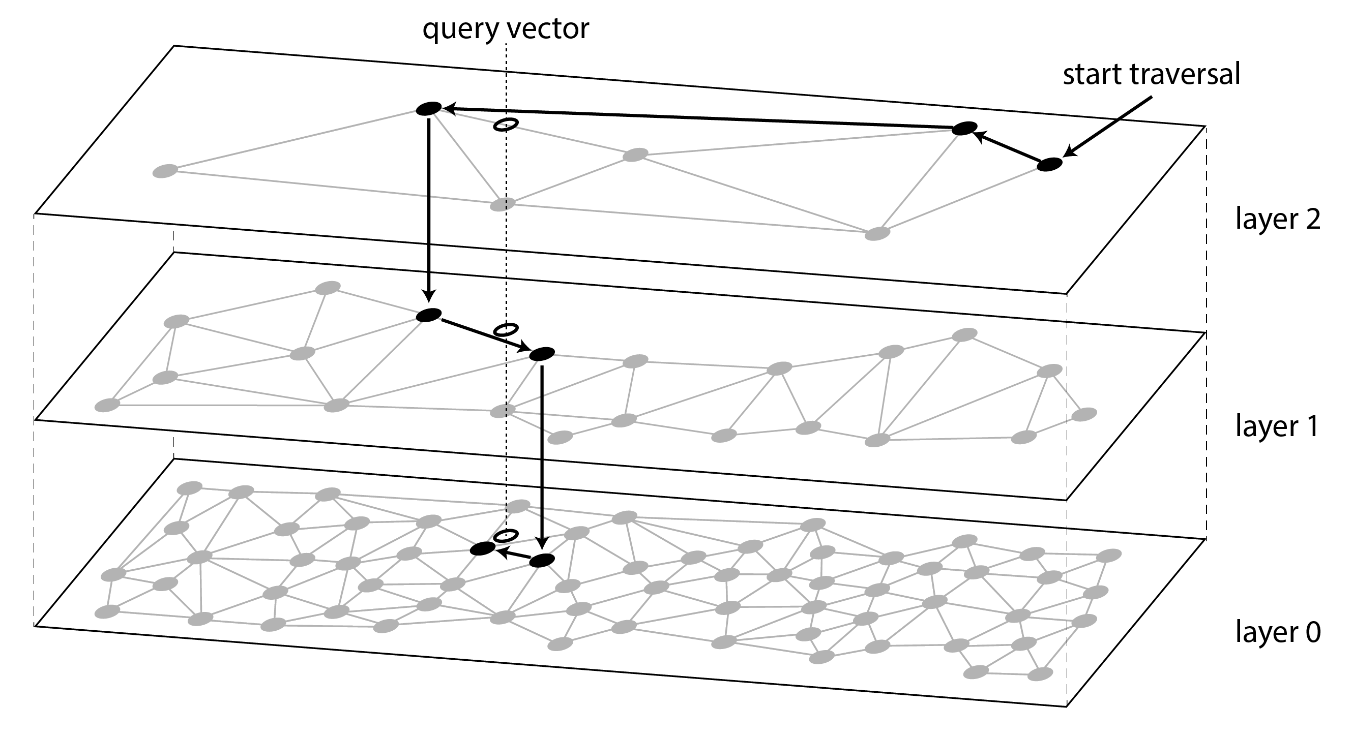
Figure 4-11 Searching for the database entry that is closest to a given query vector in a HNSW index.

Many popular vector databases implement IVF and HNSW indexes. Facebook’s Faiss library has many variations of each ¹⁰¹, and PostgreSQL’s pgvector supports both as well ¹⁰². The full details of the IVF and HNSW algorithms are beyond the scope of this book, but their papers are an excellent resource ¹⁰³ ¹⁰⁴.

Summary

In this chapter we tried to get to the bottom of how databases perform storage and retrieval. What happens when you store data in a database, and what does the database do when you query for the data again later?

“Analytical versus Operational Systems” introduced the distinction between transaction processing (OLTP) and analytics (OLAP). In this chapter we saw that storage engines optimized for OLTP look very different from those optimized for analytics:

OLTP systems are optimized for a high volume of requests, each of which reads and writes a small number of records, and which need fast responses. The records are typically accessed via a primary key or a secondary index, and these indexes are typically ordered mappings from key to record, which also support range queries.
Data warehouses and similar analytic systems are optimized for complex read queries that scan over a large number of records. They generally use a column-oriented storage layout with compression that minimizes the amount of data that such a query needs to read off disk, and just-in-time compilation of queries or vectorization to minimize the amount of CPU time spent processing the data.

On the OLTP side, we saw storage engines from two main schools of thought:

The log-structured approach, which only permits appending to files and deleting obsolete files, but never updates a file that has been written. SSTables, LSM-trees, RocksDB, Cassandra, HBase, Scylla, Lucene, and others belong to this group. In general, log-structured storage engines tend to provide high write throughput.
The update-in-place approach, which treats the disk as a set of fixed-size pages that can be overwritten. B-trees, the biggest example of this philosophy, are used in all major relational OLTP databases and also many nonrelational ones. As a rule of thumb, B-trees tend to be better for reads, providing higher read throughput and lower response times than log-structured storage.

We then looked at indexes that can search for multiple conditions at the same time: multidimensional indexes such as R-trees that can search for points on a map by latitude and longitude at the same time, and full-text search indexes that can search for multiple keywords appearing in the same text. Finally, vector databases are used for semantic search on text documents and other media; they use vectors with a larger number of dimensions and find similar documents by comparing vector similarity.

As an application developer, if you’re armed with this knowledge about the internals of storage engines, you are in a much better position to know which tool is best suited for your particular application. If you need to adjust a database’s tuning parameters, this understanding allows you to imagine what effect a higher or a lower value may have.

Although this chapter couldn’t make you an expert in tuning any one particular storage engine, it has hopefully equipped you with enough vocabulary and ideas that you can make sense of the documentation for the database of your choice.

References

Nikolay Samokhvalov. How partial, covering, and multicolumn indexes may slow down UPDATEs in PostgreSQL. postgres.ai, October 2021. Archived at perma.cc/PBK3-F4G9 ↩︎
Goetz Graefe. Modern B-Tree Techniques. Foundations and Trends in Databases, volume 3, issue 4, pages 203–402, August 2011. doi:10.1561/1900000028 ↩︎ ↩︎ ↩︎
Evan Jones. Why databases use ordered indexes but programming uses hash tables. evanjones.ca, December 2019. Archived at perma.cc/NJX8-3ZZD ↩︎
Branimir Lambov. CEP-25: Trie-indexed SSTable format. cwiki.apache.org, November 2022. Archived at perma.cc/HD7W-PW8U. Linked Google Doc archived at perma.cc/UL6C-AAAE ↩︎
Thomas H. Cormen, Charles E. Leiserson, Ronald L. Rivest, and Clifford Stein: Introduction to Algorithms, 3rd edition. MIT Press, 2009. ISBN: 978-0-262-53305-8 ↩︎ ↩︎ ↩︎
Branimir Lambov. Trie Memtables in Cassandra. Proceedings of the VLDB Endowment, volume 15, issue 12, pages 3359–3371, August 2022. doi:10.14778/3554821.3554828 ↩︎
Dhruba Borthakur. The History of RocksDB. rocksdb.blogspot.com, November 2013. Archived at perma.cc/Z7C5-JPSP ↩︎
Matteo Bertozzi. Apache HBase I/O – HFile. blog.cloudera.com, June 2012. Archived at perma.cc/U9XH-L2KL ↩︎
Fay Chang, Jeffrey Dean, Sanjay Ghemawat, Wilson C. Hsieh, Deborah A. Wallach, Mike Burrows, Tushar Chandra, Andrew Fikes, and Robert E. Gruber. Bigtable: A Distributed Storage System for Structured Data. At 7th USENIX Symposium on Operating System Design and Implementation (OSDI), November 2006. ↩︎ ↩︎
Patrick O’Neil, Edward Cheng, Dieter Gawlick, and Elizabeth O’Neil. The Log-Structured Merge-Tree (LSM-Tree). Acta Informatica, volume 33, issue 4, pages 351–385, June 1996. doi:10.1007/s002360050048 ↩︎
Mendel Rosenblum and John K. Ousterhout. The Design and Implementation of a Log-Structured File System. ACM Transactions on Computer Systems, volume 10, issue 1, pages 26–52, February 1992. doi:10.1145/146941.146943 ↩︎
Michael Armbrust, Tathagata Das, Liwen Sun, Burak Yavuz, Shixiong Zhu, Mukul Murthy, Joseph Torres, Herman van Hovell, Adrian Ionescu, Alicja Łuszczak, Michał Świtakowski, Michał Szafrański, Xiao Li, Takuya Ueshin, Mostafa Mokhtar, Peter Boncz, Ali Ghodsi, Sameer Paranjpye, Pieter Senster, Reynold Xin, and Matei Zaharia. Delta Lake: High-Performance ACID Table Storage over Cloud Object Stores. Proceedings of the VLDB Endowment, volume 13, issue 12, pages 3411–3424, August 2020. doi:10.14778/3415478.3415560 ↩︎ ↩︎
Burton H. Bloom. Space/Time Trade-offs in Hash Coding with Allowable Errors. Communications of the ACM, volume 13, issue 7, pages 422–426, July 1970. doi:10.1145/362686.362692 ↩︎
Adam Kirsch and Michael Mitzenmacher. Less Hashing, Same Performance: Building a Better Bloom Filter. Random Structures & Algorithms, volume 33, issue 2, pages 187–218, September 2008. doi:10.1002/rsa.20208 ↩︎
Thomas Hurst. Bloom Filter Calculator. hur.st, September 2023. Archived at perma.cc/L3AV-6VC2 ↩︎
Chen Luo and Michael J. Carey. LSM-based storage techniques: a survey. The VLDB Journal, volume 29, pages 393–418, July 2019. doi:10.1007/s00778-019-00555-y ↩︎
Subhadeep Sarkar and Manos Athanassoulis. Dissecting, Designing, and Optimizing LSM-based Data Stores. Tutorial at ACM International Conference on Management of Data (SIGMOD), June 2022. Slides archived at perma.cc/93B3-E827 ↩︎
Mark Callaghan. Name that compaction algorithm. smalldatum.blogspot.com, August 2018. Archived at perma.cc/CN4M-82DY ↩︎
Prashanth Rao. Embedded databases (1): The harmony of DuckDB, KùzuDB and LanceDB. thedataquarry.com, August 2023. Archived at perma.cc/PA28-2R35 ↩︎
Hacker News discussion. Bluesky migrates to single-tenant SQLite. news.ycombinator.com, October 2023. Archived at perma.cc/69LM-5P6X ↩︎
Rudolf Bayer and Edward M. McCreight. Organization and Maintenance of Large Ordered Indices. Boeing Scientific Research Laboratories, Mathematical and Information Sciences Laboratory, report no. 20, July 1970. doi:10.1145/1734663.1734671 ↩︎
Douglas Comer. The Ubiquitous B-Tree. ACM Computing Surveys, volume 11, issue 2, pages 121–137, June 1979. doi:10.1145/356770.356776 ↩︎
Alex Miller. Torn Write Detection and Protection. transactional.blog, April 2025. Archived at perma.cc/G7EB-33EW ↩︎
C. Mohan and Frank Levine. ARIES/IM: An Efficient and High Concurrency Index Management Method Using Write-Ahead Logging. At ACM International Conference on Management of Data (SIGMOD), June 1992. doi:10.1145/130283.130338 ↩︎
Hironobu Suzuki. The Internals of PostgreSQL. interdb.jp, 2017. ↩︎ ↩︎
Howard Chu. LDAP at Lightning Speed. At Build Stuff ’14, November 2014. Archived at perma.cc/GB6Z-P8YH ↩︎
Manos Athanassoulis, Michael S. Kester, Lukas M. Maas, Radu Stoica, Stratos Idreos, Anastasia Ailamaki, and Mark Callaghan. Designing Access Methods: The RUM Conjecture. At 19th International Conference on Extending Database Technology (EDBT), March 2016. doi:10.5441/002/edbt.2016.42 ↩︎
Ben Stopford. Log Structured Merge Trees. benstopford.com, February 2015. Archived at perma.cc/E5BV-KUJ6 ↩︎
Mark Callaghan. The Advantages of an LSM vs a B-Tree. smalldatum.blogspot.co.uk, January 2016. Archived at perma.cc/3TYZ-EFUD ↩︎
Oana Balmau, Florin Dinu, Willy Zwaenepoel, Karan Gupta, Ravishankar Chandhiramoorthi, and Diego Didona. SILK: Preventing Latency Spikes in Log-Structured Merge Key-Value Stores. At USENIX Annual Technical Conference, July 2019. ↩︎
Igor Canadi, Siying Dong, Mark Callaghan, et al. RocksDB Tuning Guide. github.com, 2023. Archived at perma.cc/UNY4-MK6C ↩︎
Gabriel Haas and Viktor Leis. What Modern NVMe Storage Can Do, and How to Exploit it: High-Performance I/O for High-Performance Storage Engines. Proceedings of the VLDB Endowment, volume 16, issue 9, pages 2090-2102. doi:10.14778/3598581.3598584 ↩︎
Emmanuel Goossaert. Coding for SSDs. codecapsule.com, February 2014. ↩︎
Jack Vanlightly. Is sequential IO dead in the era of the NVMe drive? jack-vanlightly.com, May 2023. Archived at perma.cc/7TMZ-TAPU ↩︎
Alibaba Cloud Storage Team. Storage System Design Analysis: Factors Affecting NVMe SSD Performance (2). alibabacloud.com, January 2019. Archived at archive.org ↩︎
Xiao-Yu Hu and Robert Haas. The Fundamental Limit of Flash Random Write Performance: Understanding, Analysis and Performance Modelling. dominoweb.draco.res.ibm.com, March 2010. Archived at perma.cc/8JUL-4ZDS ↩︎
Lanyue Lu, Thanumalayan Sankaranarayana Pillai, Andrea C. Arpaci-Dusseau, and Remzi H. Arpaci-Dusseau. WiscKey: Separating Keys from Values in SSD-conscious Storage. At 4th USENIX Conference on File and Storage Technologies (FAST), February 2016. ↩︎
Peter Zaitsev. Innodb Double Write. percona.com, August 2006. Archived at perma.cc/NT4S-DK7T ↩︎
Tomas Vondra. On the Impact of Full-Page Writes. 2ndquadrant.com, November 2016. Archived at perma.cc/7N6B-CVL3 ↩︎
Mark Callaghan. Read, write & space amplification - B-Tree vs LSM. smalldatum.blogspot.com, November 2015. Archived at perma.cc/S487-WK5P ↩︎ ↩︎
Mark Callaghan. Choosing Between Efficiency and Performance with RocksDB. At Code Mesh, November 2016. Video at youtube.com/watch?v=tgzkgZVXKB4 ↩︎
Subhadeep Sarkar, Tarikul Islam Papon, Dimitris Staratzis, Zichen Zhu, and Manos Athanassoulis. Enabling Timely and Persistent Deletion in LSM-Engines. ACM Transactions on Database Systems, volume 48, issue 3, article no. 8, August 2023. doi:10.1145/3599724 ↩︎
Lukas Fittl. Postgres vs. SQL Server: B-Tree Index Differences & the Benefit of Deduplication. pganalyze.com, April 2025. Archived at perma.cc/XY6T-LTPX ↩︎
Drew Silcock. How Postgres stores data on disk – this one’s a page turner. drew.silcock.dev, August 2024. Archived at perma.cc/8K7K-7VJ2 ↩︎
Joe Webb. Using Covering Indexes to Improve Query Performance. simple-talk.com, September 2008. Archived at perma.cc/6MEZ-R5VR ↩︎
Michael Stonebraker, Samuel Madden, Daniel J. Abadi, Stavros Harizopoulos, Nabil Hachem, and Pat Helland. The End of an Architectural Era (It’s Time for a Complete Rewrite). At 33rd International Conference on Very Large Data Bases (VLDB), September 2007. ↩︎
VoltDB Technical Overview White Paper. VoltDB, 2017. Archived at perma.cc/B9SF-SK5G ↩︎
Stephen M. Rumble, Ankita Kejriwal, and John K. Ousterhout. Log-Structured Memory for DRAM-Based Storage. At 12th USENIX Conference on File and Storage Technologies (FAST), February 2014. ↩︎
Stavros Harizopoulos, Daniel J. Abadi, Samuel Madden, and Michael Stonebraker. OLTP Through the Looking Glass, and What We Found There. At ACM International Conference on Management of Data (SIGMOD), June 2008. doi:10.1145/1376616.1376713 ↩︎
Per-Åke Larson, Cipri Clinciu, Campbell Fraser, Eric N. Hanson, Mostafa Mokhtar, Michal Nowakiewicz, Vassilis Papadimos, Susan L. Price, Srikumar Rangarajan, Remus Rusanu, and Mayukh Saubhasik. Enhancements to SQL Server Column Stores. At ACM International Conference on Management of Data (SIGMOD), June 2013. doi:10.1145/2463676.2463708 ↩︎ ↩︎
Franz Färber, Norman May, Wolfgang Lehner, Philipp Große, Ingo Müller, Hannes Rauhe, and Jonathan Dees. The SAP HANA Database – An Architecture Overview. IEEE Data Engineering Bulletin, volume 35, issue 1, pages 28–33, March 2012. ↩︎
Michael Stonebraker. The Traditional RDBMS Wisdom Is (Almost Certainly) All Wrong. Presentation at EPFL, May 2013. ↩︎ ↩︎
Adam Prout, Szu-Po Wang, Joseph Victor, Zhou Sun, Yongzhu Li, Jack Chen, Evan Bergeron, Eric Hanson, Robert Walzer, Rodrigo Gomes, and Nikita Shamgunov. Cloud-Native Transactions and Analytics in SingleStore. At ACM International Conference on Management of Data (SIGMOD), June 2022. doi:10.1145/3514221.3526055 ↩︎
Tino Tereshko and Jordan Tigani. BigQuery under the hood. cloud.google.com, January 2016. Archived at perma.cc/WP2Y-FUCF ↩︎
Wes McKinney. The Road to Composable Data Systems: Thoughts on the Last 15 Years and the Future. wesmckinney.com, September 2023. Archived at perma.cc/6L2M-GTJX ↩︎
Michael Stonebraker, Daniel J. Abadi, Adam Batkin, Xuedong Chen, Mitch Cherniack, Miguel Ferreira, Edmond Lau, Amerson Lin, Sam Madden, Elizabeth O’Neil, Pat O’Neil, Alex Rasin, Nga Tran, and Stan Zdonik. C-Store: A Column-oriented DBMS. At 31st International Conference on Very Large Data Bases (VLDB), pages 553–564, September 2005. ↩︎
Julien Le Dem. Dremel Made Simple with Parquet. blog.twitter.com, September 2013. ↩︎
Sergey Melnik, Andrey Gubarev, Jing Jing Long, Geoffrey Romer, Shiva Shivakumar, Matt Tolton, and Theo Vassilakis. Dremel: Interactive Analysis of Web-Scale Datasets. At 36th International Conference on Very Large Data Bases (VLDB), pages 330–339, September 2010. doi:10.14778/1920841.1920886 ↩︎
Joe Kearney. Understanding Record Shredding: storing nested data in columns. joekearney.co.uk, December 2016. Archived at perma.cc/ZD5N-AX5D ↩︎
Jamie Brandon. A shallow survey of OLAP and HTAP query engines. scattered-thoughts.net, September 2023. Archived at perma.cc/L3KH-J4JF ↩︎ ↩︎
Benoit Dageville, Thierry Cruanes, Marcin Zukowski, Vadim Antonov, Artin Avanes, Jon Bock, Jonathan Claybaugh, Daniel Engovatov, Martin Hentschel, Jiansheng Huang, Allison W. Lee, Ashish Motivala, Abdul Q. Munir, Steven Pelley, Peter Povinec, Greg Rahn, Spyridon Triantafyllis, and Philipp Unterbrunner. The Snowflake Elastic Data Warehouse. At ACM International Conference on Management of Data (SIGMOD), pages 215–226, June 2016. doi:10.1145/2882903.2903741 ↩︎ ↩︎
Mark Raasveldt and Hannes Mühleisen. Data Management for Data Science Towards Embedded Analytics. At 10th Conference on Innovative Data Systems Research (CIDR), January 2020. ↩︎
Jean-François Im, Kishore Gopalakrishna, Subbu Subramaniam, Mayank Shrivastava, Adwait Tumbde, Xiaotian Jiang, Jennifer Dai, Seunghyun Lee, Neha Pawar, Jialiang Li, and Ravi Aringunram. Pinot: Realtime OLAP for 530 Million Users. At ACM International Conference on Management of Data (SIGMOD), pages 583–594, May 2018. doi:10.1145/3183713.3190661 ↩︎ ↩︎
Fangjin Yang, Eric Tschetter, Xavier Léauté, Nelson Ray, Gian Merlino, and Deep Ganguli. Druid: A Real-time Analytical Data Store. At ACM International Conference on Management of Data (SIGMOD), June 2014. doi:10.1145/2588555.2595631 ↩︎ ↩︎
Chunwei Liu, Anna Pavlenko, Matteo Interlandi, and Brandon Haynes. Deep Dive into Common Open Formats for Analytical DBMSs. Proceedings of the VLDB Endowment, volume 16, issue 11, pages 3044–3056, July 2023. doi:10.14778/3611479.3611507 ↩︎ ↩︎
Xinyu Zeng, Yulong Hui, Jiahong Shen, Andrew Pavlo, Wes McKinney, and Huanchen Zhang. An Empirical Evaluation of Columnar Storage Formats. Proceedings of the VLDB Endowment, volume 17, issue 2, pages 148–161. doi:10.14778/3626292.3626298 ↩︎
Weston Pace. Lance v2: A columnar container format for modern data. blog.lancedb.com, April 2024. Archived at perma.cc/ZK3Q-S9VJ ↩︎
Yoav Helfman. Nimble, A New Columnar File Format. At VeloxCon, April 2024. ↩︎
Wes McKinney. Apache Arrow: High-Performance Columnar Data Framework. At CMU Database Group – Vaccination Database Tech Talks, December 2021. ↩︎
Wes McKinney. Python for Data Analysis, 3rd Edition. O’Reilly Media, August 2022. ISBN: 9781098104023 ↩︎
Paul Dix. The Design of InfluxDB IOx: An In-Memory Columnar Database Written in Rust with Apache Arrow. At CMU Database Group – Vaccination Database Tech Talks, May 2021. ↩︎
Carlota Soto and Mike Freedman. Building Columnar Compression for Large PostgreSQL Databases. timescale.com, March 2024. Archived at perma.cc/7KTF-V3EH ↩︎
Daniel Lemire, Gregory Ssi‐Yan‐Kai, and Owen Kaser. Consistently faster and smaller compressed bitmaps with Roaring. Software: Practice and Experience, volume 46, issue 11, pages 1547–1569, November 2016. doi:10.1002/spe.2402 ↩︎
Jaz Volpert. An entire Social Network in 1.6GB (GraphD Part 2). jazco.dev, April 2024. Archived at perma.cc/L27Z-QVMG ↩︎
Daniel J. Abadi, Peter Boncz, Stavros Harizopoulos, Stratos Idreos, and Samuel Madden. The Design and Implementation of Modern Column-Oriented Database Systems. Foundations and Trends in Databases, volume 5, issue 3, pages 197–280, December 2013. doi:10.1561/1900000024 ↩︎ ↩︎
Andrew Lamb, Matt Fuller, Ramakrishna Varadarajan, Nga Tran, Ben Vandiver, Lyric Doshi, and Chuck Bear. The Vertica Analytic Database: C-Store 7 Years Later. Proceedings of the VLDB Endowment, volume 5, issue 12, pages 1790–1801, August 2012. doi:10.14778/2367502.2367518 ↩︎
Timo Kersten, Viktor Leis, Alfons Kemper, Thomas Neumann, Andrew Pavlo, and Peter Boncz. Everything You Always Wanted to Know About Compiled and Vectorized Queries But Were Afraid to Ask. Proceedings of the VLDB Endowment, volume 11, issue 13, pages 2209–2222, September 2018. doi:10.14778/3275366.3284966 ↩︎ ↩︎
Forrest Smith. Memory Bandwidth Napkin Math. forrestthewoods.com, February 2020. Archived at perma.cc/Y8U4-PS7N ↩︎
Peter Boncz, Marcin Zukowski, and Niels Nes. MonetDB/X100: Hyper-Pipelining Query Execution. At 2nd Biennial Conference on Innovative Data Systems Research (CIDR), January 2005. ↩︎
Jingren Zhou and Kenneth A. Ross. Implementing Database Operations Using SIMD Instructions. At ACM International Conference on Management of Data (SIGMOD), pages 145–156, June 2002. doi:10.1145/564691.564709 ↩︎
Kevin Bartley. OLTP Queries: Transfer Expensive Workloads to Materialize. materialize.com, August 2024. Archived at perma.cc/4TYM-TYD8 ↩︎
Jim Gray, Surajit Chaudhuri, Adam Bosworth, Andrew Layman, Don Reichart, Murali Venkatrao, Frank Pellow, and Hamid Pirahesh. Data Cube: A Relational Aggregation Operator Generalizing Group-By, Cross-Tab, and Sub-Totals. Data Mining and Knowledge Discovery, volume 1, issue 1, pages 29–53, March 2007. doi:10.1023/A:1009726021843 ↩︎
Frank Ramsak, Volker Markl, Robert Fenk, Martin Zirkel, Klaus Elhardt, and Rudolf Bayer. Integrating the UB-Tree into a Database System Kernel. At 26th International Conference on Very Large Data Bases (VLDB), September 2000. ↩︎
Octavian Procopiuc, Pankaj K. Agarwal, Lars Arge, and Jeffrey Scott Vitter. Bkd-Tree: A Dynamic Scalable kd-Tree. At 8th International Symposium on Spatial and Temporal Databases (SSTD), pages 46–65, July 2003. doi:10.1007/978-3-540-45072-6_4 ↩︎
Joseph M. Hellerstein, Jeffrey F. Naughton, and Avi Pfeffer. Generalized Search Trees for Database Systems. At 21st International Conference on Very Large Data Bases (VLDB), September 1995. ↩︎
Isaac Brodsky. H3: Uber’s Hexagonal Hierarchical Spatial Index. eng.uber.com, June 2018. Archived at archive.org ↩︎
Robert Escriva, Bernard Wong, and Emin Gün Sirer. HyperDex: A Distributed, Searchable Key-Value Store. At ACM SIGCOMM Conference, August 2012. doi:10.1145/2377677.2377681 ↩︎
Christopher D. Manning, Prabhakar Raghavan, and Hinrich Schütze. Introduction to Information Retrieval. Cambridge University Press, 2008. ISBN: 978-0-521-86571-5, available online at nlp.stanford.edu/IR-book ↩︎
Jianguo Wang, Chunbin Lin, Yannis Papakonstantinou, and Steven Swanson. An Experimental Study of Bitmap Compression vs. Inverted List Compression. At ACM International Conference on Management of Data (SIGMOD), pages 993–1008, May 2017. doi:10.1145/3035918.3064007 ↩︎
Adrien Grand. What is in a Lucene Index? At Lucene/Solr Revolution, November 2013. Archived at perma.cc/Z7QN-GBYY ↩︎
Michael McCandless. Visualizing Lucene’s Segment Merges. blog.mikemccandless.com, February 2011. Archived at perma.cc/3ZV8-72W6 ↩︎
Lukas Fittl. Understanding Postgres GIN Indexes: The Good and the Bad. pganalyze.com, December 2021. Archived at perma.cc/V3MW-26H6 ↩︎
Jimmy Angelakos. The State of (Full) Text Search in PostgreSQL 12. At FOSDEM, February 2020. Archived at perma.cc/J6US-3WZS ↩︎
Alexander Korotkov. Index support for regular expression search. At PGConf.EU Prague, October 2012. Archived at perma.cc/5RFZ-ZKDQ ↩︎
Michael McCandless. Lucene’s FuzzyQuery Is 100 Times Faster in 4.0. blog.mikemccandless.com, March 2011. Archived at perma.cc/E2WC-GHTW ↩︎
Steffen Heinz, Justin Zobel, and Hugh E. Williams. Burst Tries: A Fast, Efficient Data Structure for String Keys. ACM Transactions on Information Systems, volume 20, issue 2, pages 192–223, April 2002. doi:10.1145/506309.506312 ↩︎
Klaus U. Schulz and Stoyan Mihov. Fast String Correction with Levenshtein Automata. International Journal on Document Analysis and Recognition, volume 5, issue 1, pages 67–85, November 2002. doi:10.1007/s10032-002-0082-8 ↩︎
Tomas Mikolov, Kai Chen, Greg Corrado, and Jeffrey Dean. Efficient Estimation of Word Representations in Vector Space. At International Conference on Learning Representations (ICLR), May 2013. doi:10.48550/arXiv.1301.3781 ↩︎
Jacob Devlin, Ming-Wei Chang, Kenton Lee, and Kristina Toutanova. BERT: Pre-training of Deep Bidirectional Transformers for Language Understanding. At Conference of the North American Chapter of the Association for Computational Linguistics: Human Language Technologies, volume 1, pages 4171–4186, June 2019. doi:10.18653/v1/N19-1423 ↩︎
Alec Radford, Karthik Narasimhan, Tim Salimans, and Ilya Sutskever. Improving Language Understanding by Generative Pre-Training. openai.com, June 2018. Archived at perma.cc/5N3C-DJ4C ↩︎
Matthijs Douze, Maria Lomeli, and Lucas Hosseini. Faiss indexes. github.com, August 2024. Archived at perma.cc/2EWG-FPBS ↩︎
Varik Matevosyan. Understanding pgvector’s HNSW Index Storage in Postgres. lantern.dev, August 2024. Archived at perma.cc/B2YB-JB59 ↩︎
Dmitry Baranchuk, Artem Babenko, and Yury Malkov. Revisiting the Inverted Indices for Billion-Scale Approximate Nearest Neighbors. At European Conference on Computer Vision (ECCV), pages 202–216, September 2018. doi:10.1007/978-3-030-01258-8_13 ↩︎
Yury A. Malkov and Dmitry A. Yashunin. Efficient and robust approximate nearest neighbor search using Hierarchical Navigable Small World graphs. IEEE Transactions on Pattern Analysis and Machine Intelligence, volume 42, issue 4, pages 824–836, April 2020. doi:10.1109/TPAMI.2018.2889473 ↩︎

5. Encoding and Evolution

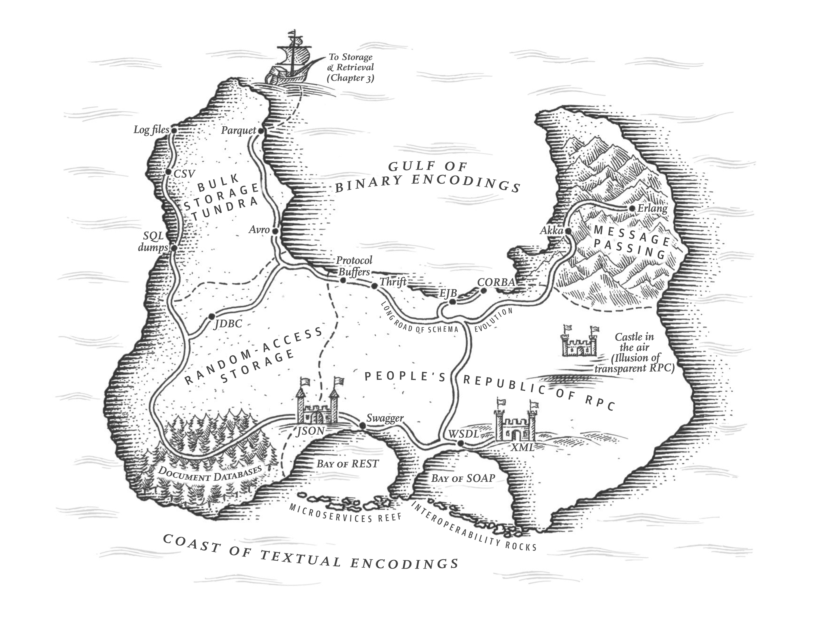
Everything changes and nothing stands still.

Heraclitus of Ephesus, as quoted by Plato in Cratylus (360 BCE)

Applications inevitably change over time. Features are added or modified as new products are launched, user requirements become better understood, or business circumstances change. In Chapter 2 we introduced the idea of evolvability: we should aim to build systems that make it easy to adapt to change (see “Evolvability: Making Change Easy”).

In most cases, a change to an application’s features also requires a change to data that it stores: perhaps a new field or record type needs to be captured, or perhaps existing data needs to be presented in a new way.

The data models we discussed in Chapter 3 have different ways of coping with such change. Relational databases generally assume that all data in the database conforms to one schema: although that schema can be changed (through schema migrations; i.e., ALTER statements), there is exactly one schema in force at any one point in time. By contrast, schema-on-read (“schemaless”) databases don’t enforce a schema, so the database can contain a mixture of older and newer data formats written at different times (see “Schema flexibility in the document model”).

When a data format or schema changes, a corresponding change to application code often needs to happen (for example, you add a new field to a record, and the application code starts reading and writing that field). However, in a large application, code changes often cannot happen instantaneously:

With server-side applications you may want to perform a rolling upgrade (also known as a staged rollout), deploying the new version to a few nodes at a time, checking whether the new version is running smoothly, and gradually working your way through all the nodes. This allows new versions to be deployed without service downtime, and thus encourages more frequent releases and better evolvability.
With client-side applications you’re at the mercy of the user, who may not install the update for some time.

This means that old and new versions of the code, and old and new data formats, may potentially all coexist in the system at the same time. In order for the system to continue running smoothly, we need to maintain compatibility in both directions:

Backward compatibility: Newer code can read data that was written by older code.
Forward compatibility: Older code can read data that was written by newer code.

Backward compatibility is normally not hard to achieve: as author of the newer code, you know the format of data written by older code, and so you can explicitly handle it (if necessary by simply keeping the old code to read the old data). Forward compatibility can be trickier, because it requires older code to ignore additions made by a newer version of the code.

Another challenge with forward compatibility is illustrated in Figure 5-1. Say you add a field to a record schema, and the newer code creates a record containing that new field and stores it in a database. Subsequently, an older version of the code (which doesn’t yet know about the new field) reads the record, updates it, and writes it back. In this situation, the desirable behavior is usually for the old code to keep the new field intact, even though it couldn’t be interpreted. But if the record is decoded into a model object that does not explicitly preserve unknown fields, data can be lost, like in Figure 5-1.

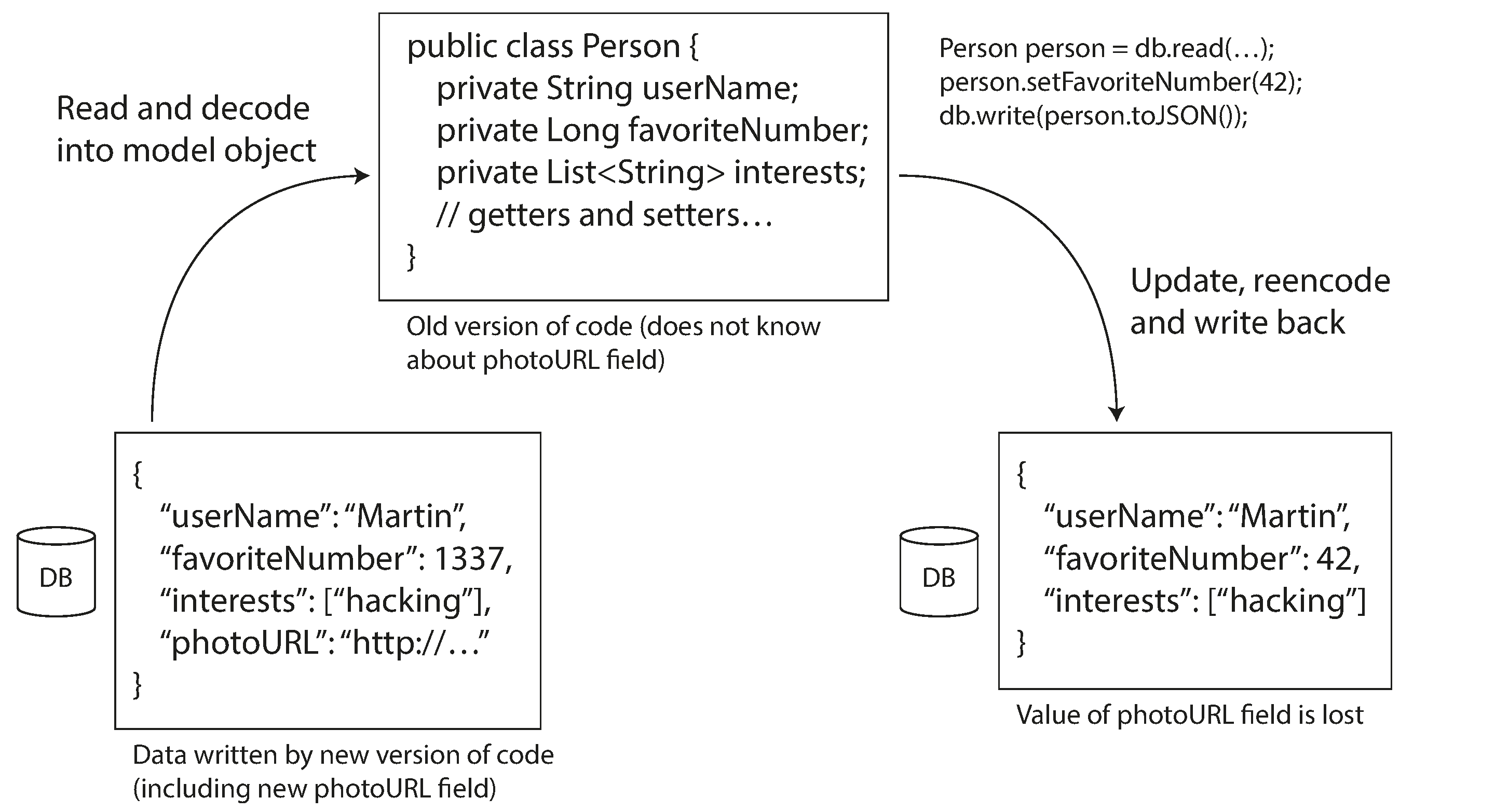
Figure 5-1 When an older version of the application updates data previously written by a newer version of the application, data may be lost if you’re not careful.

In this chapter we will look at several formats for encoding data, including JSON, XML, Protocol Buffers, and Avro. In particular, we will look at how they handle schema changes and how they support systems where old and new data and code need to coexist. We will then discuss how those formats are used for data storage and for communication: in databases, web services, REST APIs, remote procedure calls (RPC), workflow engines, and event-driven systems such as actors and message queues.

Formats for Encoding Data

Programs usually work with data in (at least) two different representations:

In memory, data is kept in objects, structs, lists, arrays, hash tables, trees, and so on. These data structures are optimized for efficient access and manipulation by the CPU (typically using pointers).
When you want to write data to a file or send it over the network, you have to encode it as some kind of self-contained sequence of bytes (for example, a JSON document). Since a pointer wouldn’t make sense to any other process, this sequence-of-bytes representation often looks quite different from the data structures that are normally used in memory.

Thus, we need some kind of translation between the two representations. The translation from the in-memory representation to a byte sequence is called encoding (also known as serialization or marshalling), and the reverse is called decoding (parsing, deserialization, unmarshalling).

TERMINOLOGY CLASH

Serialization is unfortunately also used in the context of transactions (see Chapter 8), with a completely different meaning. To avoid overloading the word we’ll stick with encoding in this book, even though serialization is perhaps a more common term.

There are exceptions in which encoding/decoding is not needed—for example, when a database operates directly on compressed data loaded from disk, as discussed in “Query Execution: Compilation and Vectorization”. There are also zero-copy data formats that are designed to be used both at runtime and on disk/on the network, without an explicit conversion step, such as Cap’n Proto and FlatBuffers.

However, most systems need to convert between in-memory objects and flat byte sequences. As this is such a common problem, there are a myriad different libraries and encoding formats to choose from. Let’s do a brief overview.

Language-Specific Formats

Many programming languages come with built-in support for encoding in-memory objects into byte sequences. For example, Java has java.io.Serializable, Python has pickle, Ruby has Marshal, and so on. Many third-party libraries also exist, such as Kryo for Java.

These encoding libraries are very convenient, because they allow in-memory objects to be saved and restored with minimal additional code. However, they also have a number of deep problems:

The encoding is often tied to a particular programming language, and reading the data in another language is very difficult. If you store or transmit data in such an encoding, you are committing yourself to your current programming language for potentially a very long time, and precluding integrating your systems with those of other organizations (which may use different languages).
In order to restore data in the same object types, the decoding process needs to be able to instantiate arbitrary classes. This is frequently a source of security problems ¹: if an attacker can get your application to decode an arbitrary byte sequence, they can instantiate arbitrary classes, which in turn often allows them to do terrible things such as remotely executing arbitrary code ² ³.
Versioning data is often an afterthought in these libraries: as they are intended for quick and easy encoding of data, they often neglect the inconvenient problems of forward and backward compatibility ⁴.
Efficiency (CPU time taken to encode or decode, and the size of the encoded structure) is also often an afterthought. For example, Java’s built-in serialization is notorious for its bad performance and bloated encoding ⁵.

For these reasons it’s generally a bad idea to use your language’s built-in encoding for anything other than very transient purposes.

JSON, XML, and Binary Variants

When moving to standardized encodings that can be written and read by many programming languages, JSON and XML are the obvious contenders. They are widely known, widely supported, and almost as widely disliked. XML is often criticized for being too verbose and unnecessarily complicated ⁶. JSON’s popularity is mainly due to its built-in support in web browsers and simplicity relative to XML. CSV is another popular language-independent format, but it only supports tabular data without nesting.

JSON, XML, and CSV are textual formats, and thus somewhat human-readable (although the syntax is a popular topic of debate). Besides the superficial syntactic issues, they also have some subtle problems:

There is a lot of ambiguity around the encoding of numbers. In XML and CSV, you cannot distinguish between a number and a string that happens to consist of digits (except by referring to an external schema). JSON distinguishes strings and numbers, but it doesn’t distinguish integers and floating-point numbers, and it doesn’t specify a precision.

This is a problem when dealing with large numbers; for example, integers greater than 2⁵³ cannot be exactly represented in an IEEE 754 double-precision floating-point number, so such numbers become inaccurate when parsed in a language that uses floating-point numbers, such as JavaScript ⁷. An example of numbers larger than 2⁵³ occurs on X (formerly Twitter), which uses a 64-bit number to identify each post. The JSON returned by the API includes post IDs twice, once as a JSON number and once as a decimal string, to work around the fact that the numbers are not correctly parsed by JavaScript applications ⁸.

JSON and XML have good support for Unicode character strings (i.e., human-readable text), but they don’t support binary strings (sequences of bytes without a character encoding). Binary strings are a useful feature, so people get around this limitation by encoding the binary data as text using Base64. The schema is then used to indicate that the value should be interpreted as Base64-encoded. This works, but it’s somewhat hacky and increases the data size by 33%.
XML Schema and JSON Schema are powerful, and thus quite complicated to learn and implement. Since the correct interpretation of data (such as numbers and binary strings) depends on information in the schema, applications that don’t use XML/JSON schemas need to potentially hard-code the appropriate encoding/decoding logic instead.
CSV does not have any schema, so it is up to the application to define the meaning of each row and column. If an application change adds a new row or column, you have to handle that change manually. CSV is also a quite vague format (what happens if a value contains a comma or a newline character?). Although its escaping rules have been formally specified ⁹, not all parsers implement them correctly.

Despite these flaws, JSON, XML, and CSV are good enough for many purposes. It’s likely that they will remain popular, especially as data interchange formats (i.e., for sending data from one organization to another). In these situations, as long as people agree on what the format is, it often doesn’t matter how pretty or efficient the format is. The difficulty of getting different organizations to agree on anything outweighs most other concerns.

JSON Schema

JSON Schema has become widely adopted as a way to model data whenever it’s exchanged between systems or written to storage. You’ll find JSON schemas in web services (see “Web services”) as part of the OpenAPI web service specification, schema registries such as Confluent’s Schema Registry and Red Hat’s Apicurio Registry, and in databases such as PostgreSQL’s pg_jsonschema validator extension and MongoDB’s $jsonSchema validator syntax.

The JSON Schema specification offers a number of features. Schemas include standard primitive types including strings, numbers, integers, objects, arrays, booleans, or nulls. But JSON Schema also offers a separate validation specification that allows developers to overlay constraints on fields. For example, a port field might have a minimum of 1 and a maximum of 65535.

JSON Schemas can have either open or closed content models. An open content model permits any field not defined in the schema to exist with any data type, whereas a closed content model only allows fields that are explicitly defined. The open content model in JSON Schema is enabled when additionalProperties is set to true, which is the default. Thus, JSON Schemas are usually a definition of what isn’t permitted (namely, invalid values on any of the defined fields), rather than what is permitted in a schema.

Open content models are powerful, but can be complex. For example, say you want to define a map from integers (such as IDs) to strings. JSON does not have a map or dictionary type, only an “object” type that can contain string keys, and values of any type. You can then constrain this type with JSON Schema so that keys may only contain digits, and values can only be strings, using patternProperties and additionalProperties as shown in Example 5-1.

Example 5-1. Example JSON Schema with integer keys and string values. Integer keys are represented as strings containing only integers since JSON Schema requires all keys to be strings.

{
    "$schema": "http://json-schema.org/draft-07/schema#",
    "type": "object",
    "patternProperties": {
        "^[0-9]+$": {
        "type": "string"
    }
    },
    "additionalProperties": false
}

In addition to open and closed content models and validators, JSON Schema supports conditional if/else schema logic, named types, references to remote schemas, and much more. All of this makes for a very powerful schema language. Such features also make for unwieldy definitions. It can be challenging to resolve remote schemas, reason about conditional rules, or evolve schemas in a forwards or backwards compatible way ¹⁰. Similar concerns apply to XML Schema ¹¹.

Binary encoding

JSON is less verbose than XML, but both still use a lot of space compared to binary formats. This observation led to the development of a profusion of binary encodings for JSON (MessagePack, CBOR, BSON, BJSON, UBJSON, BISON, Hessian, and Smile, to name a few) and for XML (WBXML and Fast Infoset, for example). These formats have been adopted in various niches, as they are more compact and sometimes faster to parse, but none of them are as widely adopted as the textual versions of JSON and XML ¹².

Some of these formats extend the set of datatypes (e.g., distinguishing integers and floating-point numbers, or adding support for binary strings), but otherwise they keep the JSON/XML data model unchanged. In particular, since they don’t prescribe a schema, they need to include all the object field names within the encoded data. That is, in a binary encoding of the JSON document in Example 5-2, they will need to include the strings userName, favoriteNumber, and interests somewhere.

Example 5-2. Example record which we will encode in several binary formats in this chapter

{
    "userName": "Martin",
    "favoriteNumber": 1337,
    "interests": ["daydreaming", "hacking"]
}

Let’s look at an example of MessagePack, a binary encoding for JSON. Figure 5-2 shows the byte sequence that you get if you encode the JSON document in Example 5-2 with MessagePack. The first few bytes are as follows:

The first byte, 0x83, indicates that what follows is an object (top four bits = 0x80) with three fields (bottom four bits = 0x03). (In case you’re wondering what happens if an object has more than 15 fields, so that the number of fields doesn’t fit in four bits, it then gets a different type indicator, and the number of fields is encoded in two or four bytes.)
The second byte, 0xa8, indicates that what follows is a string (top four bits = 0xa0) that is eight bytes long (bottom four bits = 0x08).
The next eight bytes are the field name userName in ASCII. Since the length was indicated previously, there’s no need for any marker to tell us where the string ends (or any escaping).
The next seven bytes encode the six-letter string value Martin with a prefix 0xa6, and so on.

The binary encoding is 66 bytes long, which is only a little less than the 81 bytes taken by the textual JSON encoding (with whitespace removed). All the binary encodings of JSON are similar in this regard. It’s not clear whether such a small space reduction (and perhaps a speedup in parsing) is worth the loss of human-readability.

In the following sections we will see how we can do much better, and encode the same record in just 32 bytes.

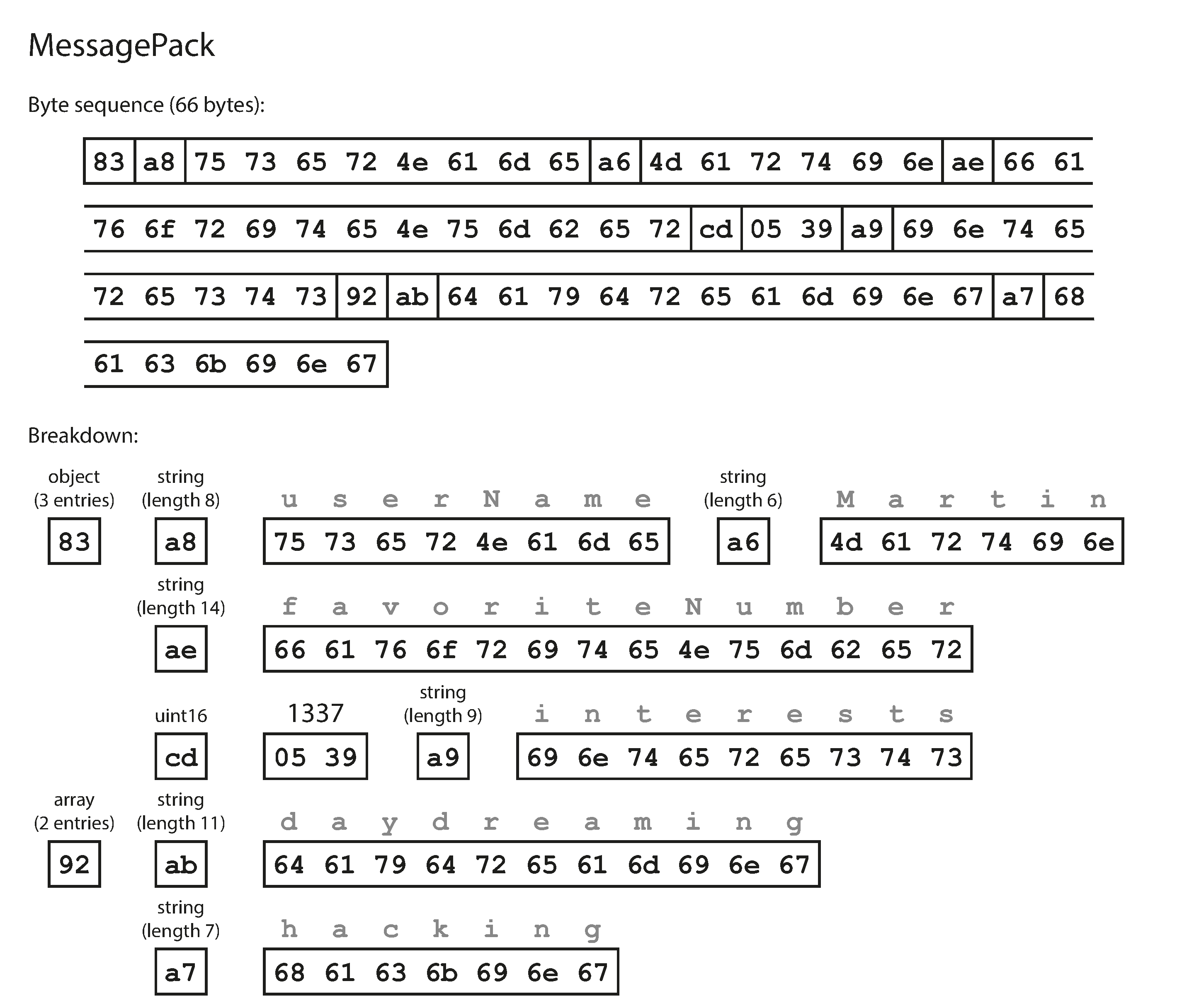
Figure 5-2 Example record Example 5-2 encoded using MessagePack.

Protocol Buffers

Protocol Buffers (protobuf) is a binary encoding library developed at Google. It is similar to Apache Thrift, which was originally developed by Facebook ¹³; most of what this section says about Protocol Buffers applies also to Thrift.

Protocol Buffers requires a schema for any data that is encoded. To encode the data in Example 5-2 in Protocol Buffers, you would describe the schema in the Protocol Buffers interface definition language (IDL) like this:

syntax = "proto3";

message Person {
    string user_name = 1;
    int64 favorite_number = 2;
    repeated string interests = 3;
}

Protocol Buffers comes with a code generation tool that takes a schema definition like the one shown here, and produces classes that implement the schema in various programming languages. Your application code can call this generated code to encode or decode records of the schema. The schema language is very simple compared to JSON Schema: it only defines the fields of records and their types, but it does not support other restrictions on the possible values of fields.

Encoding Example 5-2 using a Protocol Buffers encoder requires 33 bytes, as shown in Figure 5-3 ¹⁴.

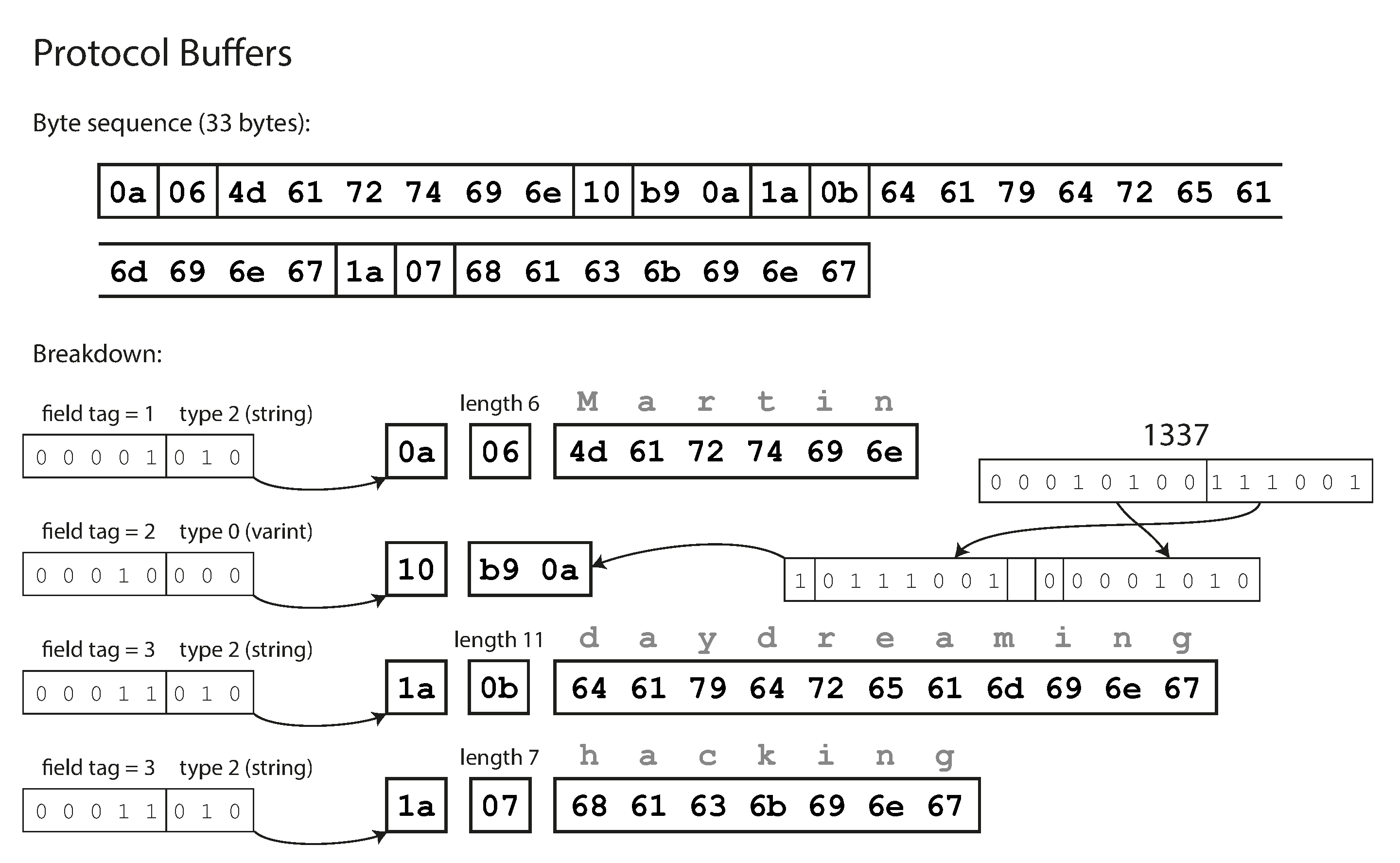
Figure 5-3 Example record encoded using Protocol Buffers.

Similarly to Figure 5-2, each field has a type annotation (to indicate whether it is a string, integer, etc.) and, where required, a length indication (such as the length of a string). The strings that appear in the data (“Martin”, “daydreaming”, “hacking”) are also encoded as ASCII (to be precise, UTF-8), similar to before.

The big difference compared to Figure 5-2 is that there are no field names (userName, favoriteNumber, interests). Instead, the encoded data contains field tags, which are numbers (1, 2, and 3). Those are the numbers that appear in the schema definition. Field tags are like aliases for fields—they are a compact way of saying what field we’re talking about, without having to spell out the field name.

As you can see, Protocol Buffers saves even more space by packing the field type and tag number into a single byte. It uses variable-length integers: the number 1337 is encoded in two bytes, with the top bit of each byte used to indicate whether there are still more bytes to come. This means numbers between –64 and 63 are encoded in one byte, numbers between –8192 and 8191 are encoded in two bytes, etc. Bigger numbers use more bytes.

Editorial note: signed integer encoding

These signed ranges describe ZigZag encoding for sint32 and sint64, not the int64 in this example. For int64, nonnegative values 0–127 use one payload byte and 128–16383 use two; negative values always use ten payload bytes, excluding the field tag. See the Protocol Buffers encoding documentation.

Protocol Buffers doesn’t have an explicit list or array datatype. Instead, the repeated modifier on the interests field indicates that the field contains a list of values, rather than a single value. In the binary encoding, the list elements are represented simply as repeated occurrences of the same field tag within the same record.

Field tags and schema evolution

We said previously that schemas inevitably need to change over time. We call this schema evolution. How does Protocol Buffers handle schema changes while keeping backward and forward compatibility?

As you can see from the examples, an encoded record is just the concatenation of its encoded fields. Each field is identified by its tag number (the numbers 1, 2, 3 in the sample schema) and annotated with a datatype (e.g., string or integer). If a field value is not set, it is simply omitted from the encoded record. From this you can see that field tags are critical to the meaning of the encoded data. You can change the name of a field in the schema, since the encoded data never refers to field names, but you cannot change a field’s tag, since that would make all existing encoded data invalid.

You can add new fields to the schema, provided that you give each field a new tag number. If old code (which doesn’t know about the new tag numbers you added) tries to read data written by new code, including a new field with a tag number it doesn’t recognize, it can simply ignore that field. The datatype annotation allows the parser to determine how many bytes it needs to skip, and preserve the unknown fields to avoid the problem in Figure 5-1. This maintains forward compatibility: old code can read records that were written by new code.

What about backward compatibility? As long as each field has a unique tag number, new code can always read old data, because the tag numbers still have the same meaning. If a field was added in the new schema, and you read old data that does not yet contain that field, it is filled in with a default value (for example, the empty string if the field type is string, or zero if it’s a number).

Removing a field is just like adding a field, with backward and forward compatibility concerns reversed. You can never use the same tag number again, because you may still have data written somewhere that includes the old tag number, and that field must be ignored by new code. Tag numbers used in the past can be reserved in the schema definition to ensure they are not forgotten.

What about changing the datatype of a field? That is possible with some types—check the documentation for details—but there is a risk that values will get truncated. For example, say you change a 32-bit integer into a 64-bit integer. New code can easily read data written by old code, because the parser can fill in any missing bits with zeros. However, if old code reads data written by new code, the old code is still using a 32-bit variable to hold the value. If the decoded 64-bit value won’t fit in 32 bits, it will be truncated.

Avro

Apache Avro is another binary encoding format that is interestingly different from Protocol Buffers. It was started in 2009 as a subproject of Hadoop, as a result of Protocol Buffers not being a good fit for Hadoop’s use cases ¹⁵.

Avro also uses a schema to specify the structure of the data being encoded. It has two schema languages: one (Avro IDL) intended for human editing, and one (based on JSON) that is more easily machine-readable. Like Protocol Buffers, this schema language specifies only fields and their types, and not complex validation rules like in JSON Schema.

Our example schema, written in Avro IDL, might look like this:

record Person {
    string                  userName;
    union { null, long }    favoriteNumber = null;
    array<string>           interests;
}

The equivalent JSON representation of that schema is as follows:

{
    "type": "record",
    "name": "Person",
    "fields": [
        {"name": "userName",        "type": "string"},
        {"name": "favoriteNumber",  "type": ["null", "long"], "default": null},
        {"name": "interests",       "type": {"type": "array", "items": "string"}}
    ]
}

First of all, notice that there are no tag numbers in the schema. If we encode our example record (Example 5-2) using this schema, the Avro binary encoding is just 32 bytes long—the most compact of all the encodings we have seen. The breakdown of the encoded byte sequence is shown in Figure 5-4.

If you examine the byte sequence, you can see that there is nothing to identify fields or their datatypes. The encoding simply consists of values concatenated together. A string is just a length prefix followed by UTF-8 bytes, but there’s nothing in the encoded data that tells you that it is a string. It could just as well be an integer, or something else entirely. An integer is encoded using a variable-length encoding.

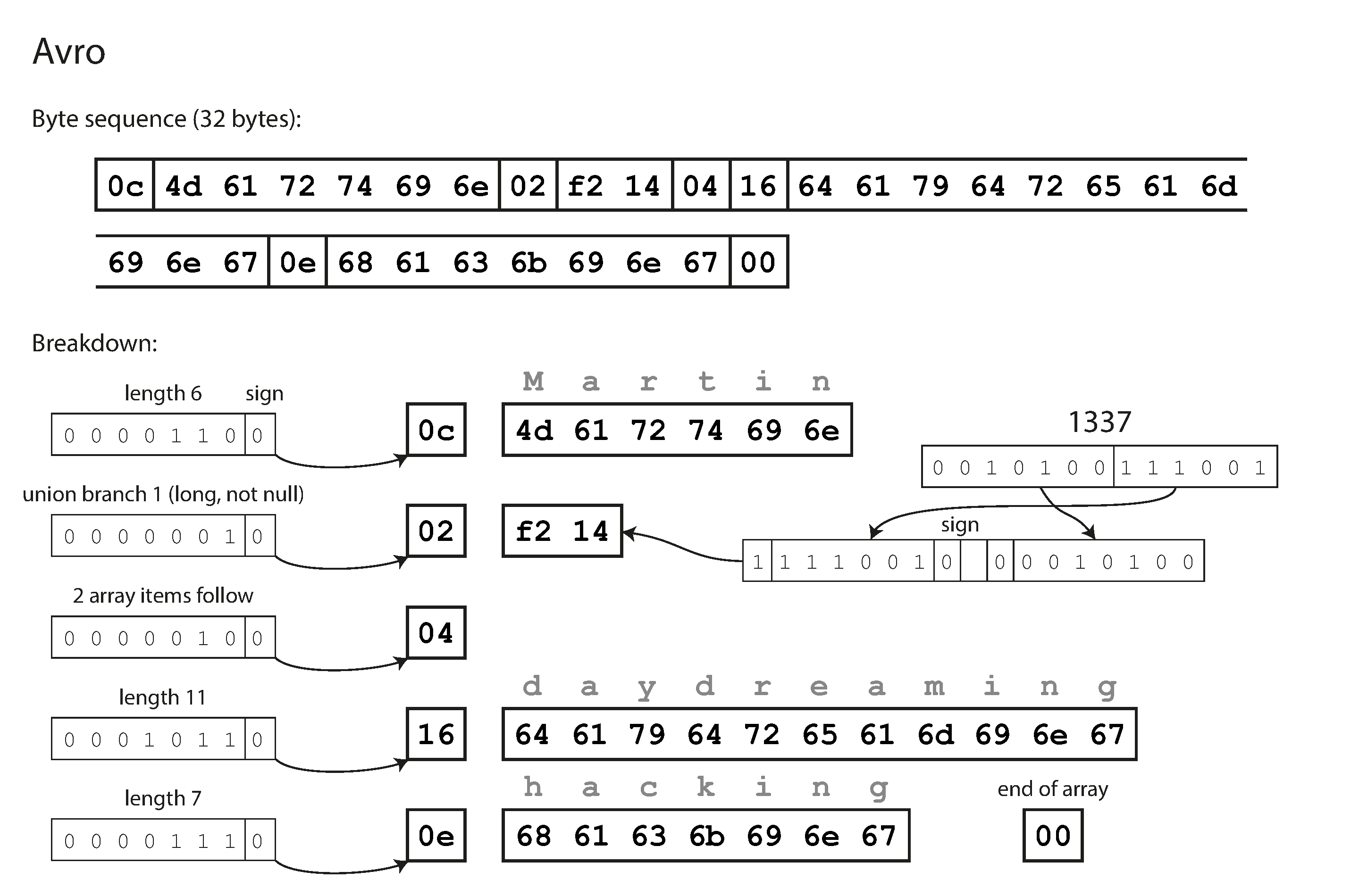
Figure 5-4 Example record encoded using Avro.

To parse the binary data, you go through the fields in the order that they appear in the schema and use the schema to tell you the datatype of each field. This means that the binary data can only be decoded correctly if the code reading the data is using the exact same schema as the code that wrote the data. Any mismatch in the schema between the reader and the writer would mean incorrectly decoded data.

So, how does Avro support schema evolution?

The writer’s schema and the reader’s schema

When an application wants to encode some data (to write it to a file or database, to send it over the network, etc.), it encodes the data using whatever version of the schema it knows about—for example, that schema may be compiled into the application. This is known as the writer’s schema.

When an application wants to decode some data (read it from a file or database, receive it from the network, etc.), it uses two schemas: the writer’s schema that is identical to the one used for encoding, and the reader’s schema, which may be different. This is illustrated in Figure 5-5. The reader’s schema defines the fields of each record that the application code is expecting, and their types.

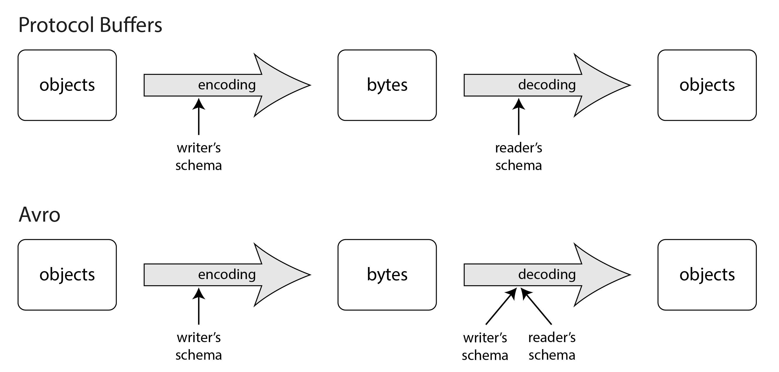
Figure 5-5 In Protocol Buffers, encoding and decoding can use different versions of a schema. In Avro, decoding uses two schemas: the writer's schema must be identical to the one used for encoding, but the reader's schema can be an older or newer version.

If the reader’s and writer’s schema are the same, decoding is easy. If they are different, Avro resolves the differences by looking at the writer’s schema and the reader’s schema side by side and translating the data from the writer’s schema into the reader’s schema. The Avro specification ¹⁶ ¹⁷ defines exactly how this resolution works, and it is illustrated in Figure 5-6.

For example, it’s no problem if the writer’s schema and the reader’s schema have their fields in a different order, because the schema resolution matches up the fields by field name. If the code reading the data encounters a field that appears in the writer’s schema but not in the reader’s schema, it is ignored. If the code reading the data expects some field, but the writer’s schema does not contain a field of that name, it is filled in with a default value declared in the reader’s schema.

Figure 5-6 An Avro reader resolves differences between the writer's schema and the reader's schema.

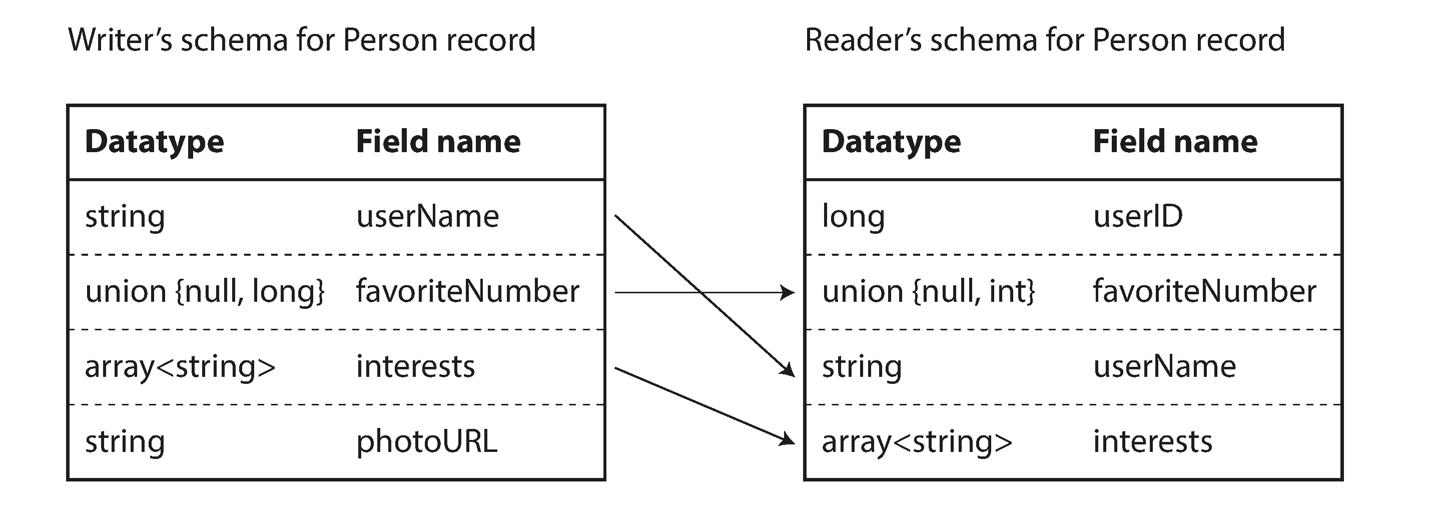
Schema evolution rules

With Avro, forward compatibility means that you can have a new version of the schema as writer and an old version of the schema as reader. Conversely, backward compatibility means that you can have a new version of the schema as reader and an old version as writer.

To maintain compatibility, you may only add or remove a field that has a default value. (The field favoriteNumber in our Avro schema has a default value of null.) For example, say you add a field with a default value, so this new field exists in the new schema but not the old one. When a reader using the new schema reads a record written with the old schema, the default value is filled in for the missing field.

If you were to add a field that has no default value, new readers wouldn’t be able to read data written by old writers, so you would break backward compatibility. If you were to remove a field that has no default value, old readers wouldn’t be able to read data written by new writers, so you would break forward compatibility.

In some programming languages, null is an acceptable default for any variable, but this is not the case in Avro: if you want to allow a field to be null, you have to use a union type. For example, union { null, long, string } field; indicates that field can be a number, or a string, or null. You can only use null as a default value if it is the first branch of the union. This is a little more verbose than having everything nullable by default, but it helps prevent bugs by being explicit about what can and cannot be null ¹⁸.

Editorial note: Avro version difference

The first-branch restriction appears in the Avro 1.11.3 specification. The Avro 1.12.0 specification, cited in this chapter, instead uses the first union branch that matches the default value; it need not be the first branch in the union. Under 1.12.0, a null default therefore needs a matching null branch. Listing it first, as in this example, remains valid.

Changing the datatype of a field is possible, provided that Avro can convert the type. Changing the name of a field is possible but a little tricky: the reader’s schema can contain aliases for field names, so it can match an old writer’s schema field names against the aliases. This means that changing a field name is backward compatible but not forward compatible. Similarly, adding a branch to a union type is backward compatible but not forward compatible.

But what is the writer’s schema?

There is an important question that we’ve glossed over so far: how does the reader know the writer’s schema with which a particular piece of data was encoded? We can’t just include the entire schema with every record, because the schema would likely be much bigger than the encoded data, making all the space savings from the binary encoding futile.

The answer depends on the context in which Avro is being used. To give a few examples:

Large file with lots of records: A common use for Avro is for storing a large file containing millions of records, all encoded with the same schema. (We will discuss this kind of situation in Chapter 11.) In this case, the writer of that file can just include the writer’s schema once at the beginning of the file. Avro specifies a file format (object container files) to do this.
Database with individually written records: In a database, different records may be written at different points in time using different writer’s schemas—you cannot assume that all the records will have the same schema. The simplest solution is to include a version number at the beginning of every encoded record, and to keep a list of schema versions in your database. A reader can fetch a record, extract the version number, and then fetch the writer’s schema for that version number from the database. Using that writer’s schema, it can decode the rest of the record.

Confluent’s schema registry for Apache Kafka ¹⁹ and LinkedIn’s Espresso ²⁰ work this way, for example.

Sending records over a network connection: When two processes are communicating over a bidirectional network connection, they can negotiate the schema version on connection setup and then use that schema for the lifetime of the connection. The Avro RPC protocol (see “Dataflow Through Services: REST and RPC”) works like this.

A database of schema versions is a useful thing to have in any case, since it acts as documentation and gives you a chance to check schema compatibility ²¹. As the version number, you could use a simple incrementing integer, or you could use a hash of the schema.

Dynamically generated schemas

One advantage of Avro’s approach, compared to Protocol Buffers, is that the schema doesn’t contain any tag numbers. But why is this important? What’s the problem with keeping a couple of numbers in the schema?

The difference is that Avro is friendlier to dynamically generated schemas. For example, say you have a relational database whose contents you want to dump to a file, and you want to use a binary format to avoid the aforementioned problems with textual formats (JSON, CSV, XML). If you use Avro, you can fairly easily generate an Avro schema (in the JSON representation we saw earlier) from the relational schema and encode the database contents using that schema, dumping it all to an Avro object container file ²². You can generate a record schema for each database table, and each column becomes a field in that record. The column name in the database maps to the field name in Avro.

Now, if the database schema changes (for example, a table has one column added and one column removed), you can just generate a new Avro schema from the updated database schema and export data in the new Avro schema. The data export process does not need to pay any attention to the schema change—it can simply do the schema conversion every time it runs. Anyone who reads the new data files will see that the fields of the record have changed, but since the fields are identified by name, the updated writer’s schema can still be matched up with the old reader’s schema.

By contrast, if you were using Protocol Buffers for this purpose, the field tags would likely have to be assigned by hand: every time the database schema changes, an administrator would have to manually update the mapping from database column names to field tags. (It might be possible to automate this, but the schema generator would have to be very careful to not assign previously used field tags.) This kind of dynamically generated schema simply wasn’t a design goal of Protocol Buffers, whereas it was for Avro.

The Merits of Schemas

As we saw, Protocol Buffers and Avro both use a schema to describe a binary encoding format. Their schema languages are much simpler than XML Schema or JSON Schema, which support much more detailed validation rules (e.g., “the string value of this field must match this regular expression” or “the integer value of this field must be between 0 and 100”). As Protocol Buffers and Avro are simpler to implement and simpler to use, they have grown to support a fairly wide range of programming languages.

The ideas on which these encodings are based are by no means new. For example, they have a lot in common with ASN.1, a schema definition language that was first standardized in 1984 ²³ ²⁴. It was used to define various network protocols, and its binary encoding (DER) is still used to encode SSL certificates (X.509), for example ²⁵. ASN.1 supports schema evolution using tag numbers, similar to Protocol Buffers ²⁶. However, it’s also very complex and badly documented, so ASN.1 is probably not a good choice for new applications.

Many data systems also implement some kind of proprietary binary encoding for their data. For example, most relational databases have a network protocol over which you can send queries to the database and get back responses. Those protocols are generally specific to a particular database, and the database vendor provides a driver (e.g., using the ODBC or JDBC APIs) that decodes responses from the database’s network protocol into in-memory data structures.

So, we can see that although textual data formats such as JSON, XML, and CSV are widespread, binary encodings based on schemas are also a viable option. They have a number of nice properties:

They can be much more compact than the various “binary JSON” variants, since they can omit field names from the encoded data.
The schema is a valuable form of documentation, and because the schema is required for decoding, you can be sure that it is up to date (whereas manually maintained documentation may easily diverge from reality).
Keeping a database of schemas allows you to check forward and backward compatibility of schema changes, before anything is deployed.
For users of statically typed programming languages, the ability to generate code from the schema is useful, since it enables type-checking at compile time.

In summary, schema evolution allows the same kind of flexibility as schemaless/schema-on-read JSON databases provide (see “Schema flexibility in the document model”), while also providing better guarantees about your data and better tooling.

Modes of Dataflow

At the beginning of this chapter we said that whenever you want to send some data to another process with which you don’t share memory—for example, whenever you want to send data over the network or write it to a file—you need to encode it as a sequence of bytes. We then discussed a variety of different encodings for doing this.

We talked about forward and backward compatibility, which are important for evolvability (making change easy by allowing you to upgrade different parts of your system independently, and not having to change everything at once). Compatibility is a relationship between one process that encodes the data, and another process that decodes it.

That’s a fairly abstract idea—there are many ways data can flow from one process to another. Who encodes the data, and who decodes it? In the rest of this chapter we will explore some of the most common ways how data flows between processes:

Via databases (see “Dataflow Through Databases”)
Via service calls (see “Dataflow Through Services: REST and RPC”)
Via workflow engines (see “Durable Execution and Workflows”)
Via asynchronous messages (see “Event-Driven Architectures”)

Dataflow Through Databases

In a database, the process that writes to the database encodes the data, and the process that reads from the database decodes it. There may just be a single process accessing the database, in which case the reader is simply a later version of the same process—in that case you can think of storing something in the database as sending a message to your future self.

Backward compatibility is clearly necessary here; otherwise your future self won’t be able to decode what you previously wrote.

In general, it’s common for several different processes to be accessing a database at the same time. Those processes might be several different applications or services, or they may simply be several instances of the same service (running in parallel for scalability or fault tolerance). Either way, in an environment where the application is changing, it is likely that some processes accessing the database will be running newer code and some will be running older code—for example because a new version is currently being deployed in a rolling upgrade, so some instances have been updated while others haven’t yet.

This means that a value in the database may be written by a newer version of the code, and subsequently read by an older version of the code that is still running. Thus, forward compatibility is also often required for databases.

Different values written at different times

A database generally allows any value to be updated at any time. This means that within a single database you may have some values that were written five milliseconds ago, and some values that were written five years ago.

When you deploy a new version of your application (of a server-side application, at least), you may entirely replace the old version with the new version within a few minutes. The same is not true of database contents: the five-year-old data will still be there, in the original encoding, unless you have explicitly rewritten it since then. This observation is sometimes summed up as data outlives code.

Rewriting (migrating) data into a new schema is certainly possible, but it’s an expensive thing to do on a large dataset, so most databases avoid it if possible. Most relational databases allow simple schema changes, such as adding a new column with a null default value, without rewriting existing data. When an old row is read, the database fills in nulls for any columns that are missing from the encoded data on disk. Schema evolution thus allows the entire database to appear as if it was encoded with a single schema, even though the underlying storage may contain records encoded with various historical versions of the schema.

More complex schema changes—for example, changing a single-valued attribute to be multi-valued, or moving some data into a separate table—still require data to be rewritten, often at the application level ²⁷. Maintaining forward and backward compatibility across such migrations is still a research problem ²⁸.

Archival storage

Perhaps you take a snapshot of your database from time to time, say for backup purposes or for loading into a data warehouse (see “Data Warehousing”). In this case, the data dump will typically be encoded using the latest schema, even if the original encoding in the source database contained a mixture of schema versions from different eras. Since you’re copying the data anyway, you might as well encode the copy of the data consistently.

As the data dump is written in one go and is thereafter immutable, formats like Avro object container files are a good fit. This is also a good opportunity to encode the data in an analytics-friendly column-oriented format such as Parquet (see “Column Compression”).

In Chapter 11 we will talk more about using data in archival storage.

Dataflow Through Services: REST and RPC

When you have processes that need to communicate over a network, there are a few different ways of arranging that communication. The most common arrangement is to have two roles: clients and servers. The servers expose an API over the network, and the clients can connect to the servers to make requests to that API. The API exposed by the server is known as a service.

The web works this way: clients (web browsers) make requests to web servers, making GET requests to download HTML, CSS, JavaScript, images, etc., and making POST requests to submit data to the server. The API consists of a standardized set of protocols and data formats (HTTP, URLs, SSL/TLS, HTML, etc.). Because web browsers, web servers, and website authors mostly agree on these standards, you can use any web browser to access any website (at least in theory!).

Web browsers are not the only type of client. For example, native apps running on mobile devices and desktop computers often talk to servers, and client-side JavaScript applications running inside web browsers can also make HTTP requests. In this case, the server’s response is typically not HTML for displaying to a human, but rather data in an encoding that is convenient for further processing by the client-side application code (most often JSON). Although HTTP may be used as the transport protocol, the API implemented on top is application-specific, and the client and server need to agree on the details of that API.

In some ways, services are similar to databases: they typically allow clients to submit and query data. However, while databases allow arbitrary queries using the query languages we discussed in Chapter 3, services expose an application-specific API that only allows inputs and outputs that are predetermined by the business logic (application code) of the service ²⁹. This restriction provides a degree of encapsulation: services can impose fine-grained restrictions on what clients can and cannot do.

A key design goal of a service-oriented/microservices architecture is to make the application easier to change and maintain by making services independently deployable and evolvable. A common principle is that each service should be owned by one team, and that team should be able to release new versions of the service frequently, without having to coordinate with other teams. We should therefore expect old and new versions of servers and clients to be running at the same time, and so the data encoding used by servers and clients must be compatible across versions of the service API.

Web services

When HTTP is used as the underlying protocol for talking to the service, it is called a web service. Web services are commonly used when building a service oriented or microservices architecture (discussed earlier in “Microservices and Serverless”). The term “web service” is perhaps a slight misnomer, because web services are not only used on the web, but in several different contexts. For example:

A client application running on a user’s device (e.g., a native app on a mobile device, or a JavaScript web app in a browser) making requests to a service over HTTP. These requests typically go over the public internet.
One service making requests to another service owned by the same organization, often located within the same datacenter, as part of a service-oriented/microservices architecture.
One service making requests to a service owned by a different organization, usually via the internet. This is used for data exchange between different organizations’ backend systems. This category includes public APIs provided by online services, such as credit card processing systems, or OAuth for shared access to user data.

The most popular service design philosophy is REST, which builds upon the principles of HTTP ³⁰ ³¹. It emphasizes simple data formats, using URLs for identifying resources and using HTTP features for cache control, authentication, and content type negotiation. An API designed according to the principles of REST is called RESTful.

Code that needs to invoke a web service API must know which HTTP endpoint to query, and what data format to send and expect in response. Even if a service adopts RESTful design principles, clients need to somehow find out these details. Service developers often use an interface definition language (IDL) to define and document their service’s API endpoints and data models, and to evolve them over time. Other developers can then use the service definition to determine how to query the service. The two most popular service IDLs are OpenAPI (also known as Swagger ³²) and gRPC. OpenAPI is used for web services that send and receive JSON data, while gRPC services send and receive Protocol Buffers.

Developers typically write OpenAPI service definitions in JSON or YAML; see Example 5-3. The service definition allows developers to define service endpoints, documentation, versions, data models, and much more. gRPC definitions look similar, but are defined using Protocol Buffers service definitions.

Example 5-3. Example OpenAPI service definition in YAML

openapi: 3.0.0
info:
  title: Ping, Pong
  version: 1.0.0
servers:
  - url: http://localhost:8080
paths:
  /ping:
    get:
      summary: Given a ping, returns a pong message
      responses:
        '200':
          description: A pong
          content:
            application/json:
              schema:
                type: object
                properties:
                  message:
                    type: string
                    example: Pong!

Even if a design philosophy and IDL are adopted, developers must still write the code that implements their service’s API calls. A service framework is often adopted to simplify this effort. Service frameworks such as Spring Boot, FastAPI, and gRPC allow developers to write the business logic for each API endpoint while the framework code handles routing, metrics, caching, authentication, and so on. Example 5-4 shows an example Python implementation of the service defined in Example 5-3.

Example 5-4. Example FastAPI service implementing the definition from Example 5-3

from fastapi import FastAPI
from pydantic import BaseModel

app = FastAPI(title="Ping, Pong", version="1.0.0")

class PongResponse(BaseModel):
    message: str = "Pong!"

@app.get("/ping", response_model=PongResponse,
         summary="Given a ping, returns a pong message")
async def ping():
    return PongResponse()

Many frameworks couple service definitions and server code together. In some cases, such as with the popular Python FastAPI framework, servers are written in code and an IDL is generated automatically. In other cases, such as with gRPC, the service definition is written first, and server code scaffolding is generated. Both approaches allow developers to generate client libraries and SDKs in a variety of languages from the service definition. In addition to code generation, IDL tools such as Swagger’s can generate documentation, verify schema change compatibility, and provide a graphical user interfaces for developers to query and test services.

The problems with remote procedure calls (RPCs)

Web services are merely the latest incarnation of a long line of technologies for making API requests over a network, many of which received a lot of hype but have serious problems. Enterprise JavaBeans (EJB) and Java’s Remote Method Invocation (RMI) are limited to Java. The Distributed Component Object Model (DCOM) is limited to Microsoft platforms. The Common Object Request Broker Architecture (CORBA) is excessively complex, and does not provide backward or forward compatibility ³³. SOAP and the WS-* web services framework aim to provide interoperability across vendors, but are also plagued by complexity and compatibility problems ³⁴ ³⁵ ³⁶.

All of these are based on the idea of a remote procedure call (RPC), which has been around since the 1970s ³⁷. The RPC model tries to make a request to a remote network service look the same as calling a function or method in your programming language, within the same process (this abstraction is called location transparency). Although RPC seems convenient at first, the approach is fundamentally flawed ³⁸ ³⁹. A network request is very different from a local function call:

A local function call is predictable and either succeeds or fails, depending only on parameters that are under your control. A network request is unpredictable: the request or response may be lost due to a network problem, or the remote machine may be slow or unavailable, and such problems are entirely outside of your control. Network problems are common, so you have to anticipate them, for example by retrying a failed request.
A local function call either returns a result, or throws an exception, or never returns (because it goes into an infinite loop or the process crashes). A network request has another possible outcome: it may return without a result, due to a timeout. In that case, you simply don’t know what happened: if you don’t get a response from the remote service, you have no way of knowing whether the request got through or not. (We discuss this issue in more detail in Chapter 9.)
If you retry a failed network request, it could happen that the previous request actually got through, and only the response was lost. In that case, retrying will cause the action to be performed multiple times, unless you build a mechanism for deduplication (idempotence) into the protocol ⁴⁰. Local function calls don’t have this problem. (We discuss idempotence in more detail in “Idempotence”.)
Every time you call a local function, it normally takes about the same time to execute. A network request is much slower than a function call, and its latency is also wildly variable: at good times it may complete in less than a millisecond, but when the network is congested or the remote service is overloaded it may take many seconds to do exactly the same thing.
When you call a local function, you can efficiently pass it references (pointers) to objects in local memory. When you make a network request, all those parameters need to be encoded into a sequence of bytes that can be sent over the network. That’s okay if the parameters are immutable primitives like numbers or short strings, but it quickly becomes problematic with larger amounts of data and mutable objects.
The client and the service may be implemented in different programming languages, so the RPC framework must translate datatypes from one language into another. This can end up ugly, since not all languages have the same types—recall JavaScript’s problems with numbers greater than 2⁵³, for example (see “JSON, XML, and Binary Variants”). This problem doesn’t exist in a single process written in a single language.

All of these factors mean that there’s no point trying to make a remote service look too much like a local object in your programming language, because it’s a fundamentally different thing. Part of the appeal of REST is that it treats state transfer over a network as a process that is distinct from a function call.

Load balancers, service discovery, and service meshes

All services communicate over the network. For this reason, a client must know the address of the service it’s connecting to—a problem known as service discovery. The simplest approach is to configure a client to connect to the IP address and port where the service is running. This configuration will work, but if the server goes offline, is transferred to a new machine, or becomes overloaded, the client has to be manually reconfigured.

To provide higher availability and scalability, there are usually multiple instances of a service running on different machines, any of which can handle an incoming request. Spreading requests across these instances is called load balancing ⁴¹. There are many load balancing and service discovery solutions available:

Hardware load balancers are specialized pieces of equipment that are installed in data centers. They allow clients to connect to a single host and port, and incoming connections are routed to one of the servers running the service. Such load balancers detect network failures when connecting to a downstream server and shift the traffic to other servers.
Software load balancers behave in much the same way as hardware load balancers. But rather than requiring a special appliance, software load balancers such as Nginx and HAProxy are applications that can be installed on a standard machine.
The domain name service (DNS) is how domain names are resolved on the Internet when you open a webpage. It supports load balancing by allowing multiple IP addresses to be associated with a single domain name. Clients can then be configured to connect to a service using a domain name rather than IP address, and the client’s network layer picks which IP address to use when making a connection. One drawback of this approach is that DNS is designed to propagate changes over longer periods of time, and to cache DNS entries. If servers are started, stopped, or moved frequently, clients might see stale IP addresses that no longer have a server running on them.
Service discovery systems use a centralized registry rather than DNS to track which service endpoints are available. When a new service instance starts up, it registers itself with the service discovery system by declaring the host and port it’s listening on, along with relevant metadata such as shard ownership information (see Chapter 7), data center location, and more. The service then periodically sends a heartbeat signal to the discovery system to signal that the service is still available.

When a client wishes to connect to a service, it first queries the discovery system to get a list of available endpoints, and then connects directly to the endpoint. Compared to DNS, service discovery supports a much more dynamic environment where service instances change frequently. Discovery systems also give clients more metadata about the service they’re connecting to, which enables clients to make smarter load balancing decisions.

Service meshes are a sophisticated form of load balancing that combine software load balancers and service discovery. Unlike traditional software load balancers, which run on a separate machine, service mesh load balancers are typically deployed as an in-process client library or as a process or “sidecar” container on both the client and server. Client applications connect to their own local service load balancer, which connects to the server’s load balancer. From there, the connection is routed to the local server process.

Though complicated, this topology offers a number of advantages. Because the clients and servers are routed entirely through local connections, connection encryption can be handled entirely at the load balancer level. This shields clients and servers from having to deal with the complexities of SSL certificates and TLS. Mesh systems also provide sophisticated observability. They can track which services are calling each other in realtime, detect failures, track traffic load, and more.

Which solution is appropriate depends on an organization’s needs. Those running in a very dynamic service environment with an orchestrator such as Kubernetes often choose to run a service mesh such as Istio or Linkerd. Specialized infrastructure such as databases or messaging systems might require their own purpose-built load balancer. Simpler deployments are best served with software load balancers.

Data encoding and evolution for RPC

For evolvability, it is important that RPC clients and servers can be changed and deployed independently. Compared to data flowing through databases (as described in the last section), we can make a simplifying assumption in the case of dataflow through services: it is reasonable to assume that all the servers will be updated first, and all the clients second. Thus, you only need backward compatibility on requests, and forward compatibility on responses.

The backward and forward compatibility properties of an RPC scheme are inherited from whatever encoding it uses:

gRPC (Protocol Buffers) and Avro RPC can be evolved according to the compatibility rules of the respective encoding format.
RESTful APIs most commonly use JSON for responses, and JSON or URI-encoded/form-encoded request parameters for requests. Adding optional request parameters and adding new fields to response objects are usually considered changes that maintain compatibility.

Service compatibility is made harder by the fact that RPC is often used for communication across organizational boundaries, so the provider of a service often has no control over its clients and cannot force them to upgrade. Thus, compatibility needs to be maintained for a long time, perhaps indefinitely. If a compatibility-breaking change is required, the service provider often ends up maintaining multiple versions of the service API side by side.

There is no agreement on how API versioning should work (i.e., how a client can indicate which version of the API it wants to use ⁴²). For RESTful APIs, common approaches are to use a version number in the URL or in the HTTP Accept header. For services that use API keys to identify a particular client, another option is to store a client’s requested API version on the server and to allow this version selection to be updated through a separate administrative interface ⁴³.

Durable Execution and Workflows

By definition, service-based architectures have multiple services that are all responsible for different portions of an application. Consider a payment processing application that charges a credit card and deposits the funds into a bank account. This system would likely have different services responsible for fraud detection, credit card integration, bank integration, and so on.

Processing a single payment in our example requires many service calls. A payment processor service might invoke the fraud detection service to check for fraud, call the credit card service to debit the credit card, and call the banking service to deposit debited funds, as shown in Figure 5-7. We call this sequence of steps a workflow, and each step a task. Workflows are typically defined as a graph of tasks. Workflow definitions may be written in a general-purpose programming language, a domain specific language (DSL), or a markup language such as Business Process Execution Language (BPEL) ⁴⁴.

TASKS, ACTIVITIES, AND FUNCTIONS

Different workflow engines use different names for tasks. Temporal, for example, uses the term activity. Others refer to tasks as durable functions. Though the names differ, the concepts are the same.

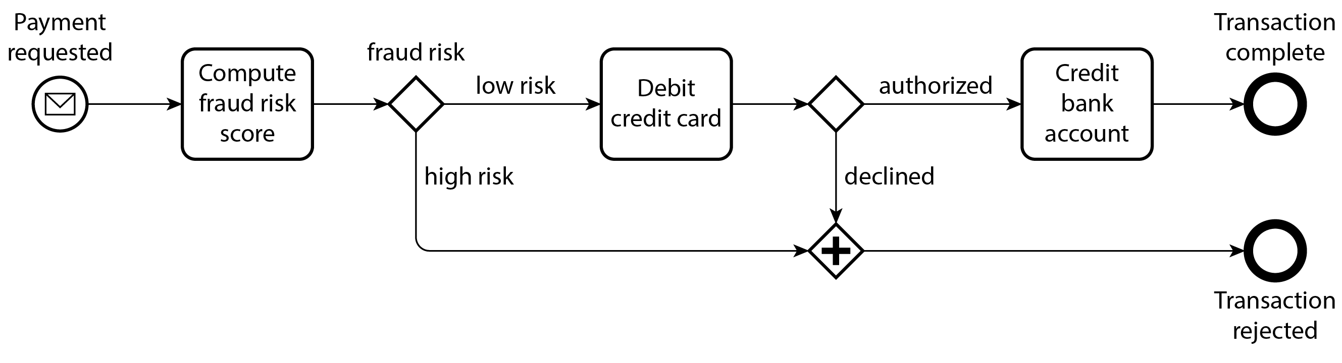
Figure 5-7 Example of a workflow expressed using Business Process Model and Notation (BPMN), a graphical notation.

Workflows are run, or executed, by a workflow engine. Workflow engines determine when to run each task, on which machine a task must be run, what to do if a task fails (e.g., if the machine crashes while the task is running), how many tasks are allowed to execute in parallel, and more.

Workflow engines are typically composed of an orchestrator and an executor. The orchestrator is responsible for scheduling tasks to be executed and the executor is responsible for executing tasks. Execution begins when a workflow is triggered. The orchestrator triggers the workflow itself if users define a time-based schedule, such as hourly execution. External sources such as a web service or even a human can also trigger workflow executions. Once triggered, executors are invoked to run tasks.

There are many kinds of workflow engines that address a diverse set of use cases. Some, such as Airflow, Dagster, and Prefect, integrate with data systems and orchestrate ETL tasks. Others, such as Camunda and Orkes, provide a graphical notation for workflows (such as BPMN, used in Figure 5-7) so that non-engineers can more easily define and execute workflows. Still others, such as Temporal and Restate provide durable execution.

Durable execution

Durable execution frameworks have become a popular way to build service-based architectures that require transactionality. In our payment example, we would like to process each payment exactly once. A failure while the workflow is executing could result in a credit card charge, but no corresponding bank account deposit. In a service-based architecture, we can’t simply wrap the two tasks in a database transaction. Moreover, we might be interacting with third-party payment gateways that we have limited control over.

Durable execution frameworks are a way to provide exactly-once semantics for workflows. If a task fails, the framework will re-execute the task, but will skip any RPC calls or state changes that the task made successfully before failing. Instead, the framework will pretend to make the call, but will instead return the results from the previous call. This is possible because durable execution frameworks log all RPCs and state changes to durable storage like a write-ahead log ⁴⁵ ⁴⁶. Example 5-5 shows an example of a workflow definition that supports durable execution using Temporal.

Example 5-5. A Temporal workflow definition fragment for the payment workflow in Figure 5-7.

@workflow.defn
class PaymentWorkflow:
    @workflow.run
    async def run(self, payment: PaymentRequest) -> PaymentResult:
        is_fraud = await workflow.execute_activity(
            check_fraud,
            payment,
            start_to_close_timeout=timedelta(seconds=15),
        )
        if is_fraud:
            return PaymentResultFraudulent
        credit_card_response = await workflow.execute_activity(
            debit_credit_card,
            payment,
            start_to_close_timeout=timedelta(seconds=15),
        )
        # ...

Frameworks like Temporal are not without their challenges. External services, such as the third-party payment gateway in our example, must still provide an idempotent API. Developers must remember to use unique IDs for these APIs to prevent duplicate execution ⁴⁷. And because durable execution frameworks log each RPC call in order, it expects a subsequent execution to make the same RPC calls in the same order. This makes code changes brittle: you might introduce undefined behavior simply by re-ordering function calls ⁴⁸. Instead of modifying the code of an existing workflow, it is safer to deploy a new version of the code separately, so that re-executions of existing workflow invocations continue to use the old version, and only new invocations use the new code ⁴⁹.

Similarly, because durable execution frameworks expect to replay all code deterministically (the same inputs produce the same outputs), nondeterministic code such as random number generators or system clocks are problematic ⁴⁸. Frameworks often provide their own, deterministic implementations of such library functions, but you have to remember to use them. In some cases, such as with Temporal’s workflowcheck tool, frameworks provide static analysis tools to determine if nondeterministic behavior has been introduced.

Note

Making code deterministic is a powerful idea, but tricky to do robustly. In “The Power of Determinism” we will return to this topic.

Event-Driven Architectures

In this final section, we will briefly look at event-driven architectures, which are another way how encoded data can flow from one process to another. A request is called an event or message; unlike RPC, the sender usually does not wait for the recipient to process the event. Moreover, events are typically not sent to the recipient via a direct network connection, but go via an intermediary called a message broker (also called an event broker, message queue, or message-oriented middleware), which stores the message temporarily. ⁵⁰.

Using a message broker has several advantages compared to direct RPC:

It can act as a buffer if the recipient is unavailable or overloaded, and thus improve system reliability.
It can automatically redeliver messages to a process that has crashed, and thus prevent messages from being lost.
It avoids the need for service discovery, since senders do not need to directly connect to the IP address of the recipient.
It allows the same message to be sent to several recipients.
It logically decouples the sender from the recipient (the sender just publishes messages and doesn’t care who consumes them).

The communication via a message broker is asynchronous: the sender doesn’t wait for the message to be delivered, but simply sends it and then forgets about it. It’s possible to implement a synchronous RPC-like model by having the sender wait for a response on a separate channel.

Message brokers

In the past, the landscape of message brokers was dominated by commercial enterprise software from companies such as TIBCO, IBM WebSphere, and webMethods, before open source implementations such as RabbitMQ, ActiveMQ, HornetQ, NATS, and Apache Kafka become popular. More recently, cloud services such as Amazon Kinesis, Azure Service Bus, and Google Cloud Pub/Sub have gained adoption. We will compare them in more detail in “Messaging Systems”.

The detailed delivery semantics vary by implementation and configuration, but in general, two message distribution patterns are most often used:

One process adds a message to a named queue, and the broker delivers that message to a consumer of that queue. If there are multiple consumers, one of them receives the message.
One process publishes a message to a named topic, and the broker delivers that message to all subscribers of that topic. If there are multiple subscribers, they all receive the message.

Message brokers typically don’t enforce any particular data model—a message is just a sequence of bytes with some metadata, so you can use any encoding format. A common approach is to use Protocol Buffers, Avro, or JSON, and to deploy a schema registry alongside the message broker to store all the valid schema versions and check their compatibility ¹⁹ ²¹. AsyncAPI, a messaging-based equivalent of OpenAPI, can also be used to specify the schema of messages.

Message brokers differ in terms of how durable their messages are. Many write messages to disk, so that they are not lost in case the message broker crashes or needs to be restarted. Unlike databases, many message brokers automatically delete messages again after they have been consumed. Some brokers can be configured to store messages indefinitely, which you would require if you want to use event sourcing (see “Event Sourcing and CQRS”).

If a consumer republishes messages to another topic, you may need to be careful to preserve unknown fields, to prevent the issue described previously in the context of databases (Figure 5-1).

Distributed actor frameworks

The actor model is a programming model for concurrency in a single process. Rather than dealing directly with threads (and the associated problems of race conditions, locking, and deadlock), logic is encapsulated in actors. Each actor typically represents one client or entity, it may have some local state (which is not shared with any other actor), and it communicates with other actors by sending and receiving asynchronous messages. Message delivery is not guaranteed: in certain error scenarios, messages will be lost. Since each actor processes only one message at a time, it doesn’t need to worry about threads, and each actor can be scheduled independently by the framework.

In distributed actor frameworks such as Akka, Orleans ⁵¹, and Erlang/OTP, this programming model is used to scale an application across multiple nodes. The same message-passing mechanism is used, no matter whether the sender and recipient are on the same node or different nodes. If they are on different nodes, the message is transparently encoded into a byte sequence, sent over the network, and decoded on the other side.

Location transparency works better in the actor model than in RPC, because the actor model already assumes that messages may be lost, even within a single process. Although latency over the network is likely higher than within the same process, there is less of a fundamental mismatch between local and remote communication when using the actor model.

A distributed actor framework essentially integrates a message broker and the actor programming model into a single framework. However, if you want to perform rolling upgrades of your actor-based application, you still have to worry about forward and backward compatibility, as messages may be sent from a node running the new version to a node running the old version, and vice versa. This can be achieved by using one of the encodings discussed in this chapter.

Summary

In this chapter we looked at several ways of turning data structures into bytes on the network or bytes on disk. We saw how the details of these encodings affect not only their efficiency, but more importantly also the architecture of applications and your options for evolving them.

In particular, many services need to support rolling upgrades, where a new version of a service is gradually deployed to a few nodes at a time, rather than deploying to all nodes simultaneously. Rolling upgrades allow new versions of a service to be released without downtime (thus encouraging frequent small releases over rare big releases) and make deployments less risky (allowing faulty releases to be detected and rolled back before they affect a large number of users). These properties are hugely beneficial for evolvability, the ease of making changes to an application.

During rolling upgrades, or for various other reasons, we must assume that different nodes are running the different versions of our application’s code. Thus, it is important that all data flowing around the system is encoded in a way that provides backward compatibility (new code can read old data) and forward compatibility (old code can read new data).

We discussed several data encoding formats and their compatibility properties:

Programming language–specific encodings are restricted to a single programming language and often fail to provide forward and backward compatibility.
Textual formats like JSON, XML, and CSV are widespread, and their compatibility depends on how you use them. They have optional schema languages, which are sometimes helpful and sometimes a hindrance. These formats are somewhat vague about datatypes, so you have to be careful with things like numbers and binary strings.
Binary schema–driven formats like Protocol Buffers and Avro allow compact, efficient encoding with clearly defined forward and backward compatibility semantics. The schemas can be useful for documentation and code generation in statically typed languages. However, these formats have the downside that data needs to be decoded before it is human-readable.

We also discussed several modes of dataflow, illustrating different scenarios in which data encodings are important:

Databases, where the process writing to the database encodes the data and the process reading from the database decodes it
RPC and REST APIs, where the client encodes a request, the server decodes the request and encodes a response, and the client finally decodes the response
Event-driven architectures (using message brokers or actors), where nodes communicate by sending each other messages that are encoded by the sender and decoded by the recipient

We can conclude that with a bit of care, backward/forward compatibility and rolling upgrades are quite achievable. May your application’s evolution be rapid and your deployments be frequent.

References

CWE-502: Deserialization of Untrusted Data. Common Weakness Enumeration, cwe.mitre.org, July 2006. Archived at perma.cc/26EU-UK9Y ↩︎
Steve Breen. What Do WebLogic, WebSphere, JBoss, Jenkins, OpenNMS, and Your Application Have in Common? This Vulnerability. foxglovesecurity.com, November 2015. Archived at perma.cc/9U97-UVVD ↩︎
Patrick McKenzie. What the Rails Security Issue Means for Your Startup. kalzumeus.com, January 2013. Archived at perma.cc/2MBJ-7PZ6 ↩︎
Brian Goetz. Towards Better Serialization. openjdk.org, June 2019. Archived at perma.cc/UK6U-GQDE ↩︎
Eishay Smith. jvm-serializers wiki. github.com, October 2023. Archived at perma.cc/PJP7-WCNG ↩︎
XML Is a Poor Copy of S-Expressions. wiki.c2.com, May 2013. Archived at perma.cc/7FAN-YBKL ↩︎
Julia Evans. Examples of floating point problems. jvns.ca, January 2023. Archived at perma.cc/M57L-QKKW ↩︎
Matt Harris. Snowflake: An Update and Some Very Important Information. Email to Twitter Development Talk mailing list, October 2010. Archived at perma.cc/8UBV-MZ3D ↩︎
Yakov Shafranovich. RFC 4180: Common Format and MIME Type for Comma-Separated Values (CSV) Files. IETF, October 2005. ↩︎
Andy Coates. Evolving JSON Schemas - Part I and Part II. creekservice.org, January 2024. Archived at perma.cc/MZW3-UA54 and perma.cc/GT5H-WKZ5 ↩︎
Pierre Genevès, Nabil Layaïda, and Vincent Quint. Ensuring Query Compatibility with Evolving XML Schemas. INRIA Technical Report 6711, November 2008. ↩︎
Tim Bray. Bits On the Wire. tbray.org, November 2019. Archived at perma.cc/3BT3-BQU3 ↩︎
Mark Slee, Aditya Agarwal, and Marc Kwiatkowski. Thrift: Scalable Cross-Language Services Implementation. Facebook technical report, April 2007. Archived at perma.cc/22BS-TUFB ↩︎
Martin Kleppmann. Schema Evolution in Avro, Protocol Buffers and Thrift. martin.kleppmann.com, December 2012. Archived at perma.cc/E4R2-9RJT ↩︎
Doug Cutting, Chad Walters, Jim Kellerman, et al. [PROPOSAL] New Subproject: Avro. Email thread on hadoop-general mailing list, lists.apache.org, April 2009. Archived at perma.cc/4A79-BMEB ↩︎
Apache Software Foundation. Apache Avro 1.12.0 Specification. avro.apache.org, August 2024. Archived at perma.cc/C36P-5EBQ ↩︎
Apache Software Foundation. Avro schemas as LL(1) CFG definitions. avro.apache.org, August 2024. Archived at perma.cc/JB44-EM9Q ↩︎
Tony Hoare. Null References: The Billion Dollar Mistake. Talk at QCon London, March 2009. ↩︎
Confluent, Inc. Schema Registry Overview. docs.confluent.io, 2024. Archived at perma.cc/92C3-A9JA ↩︎ ↩︎
Aditya Auradkar and Tom Quiggle. Introducing Espresso—LinkedIn’s Hot New Distributed Document Store. engineering.linkedin.com, January 2015. Archived at perma.cc/FX4P-VW9T ↩︎
Jay Kreps. Putting Apache Kafka to Use: A Practical Guide to Building a Stream Data Platform (Part 2). confluent.io, February 2015. Archived at perma.cc/8UA4-ZS5S ↩︎ ↩︎
Gwen Shapira. The Problem of Managing Schemas. oreilly.com, November 2014. Archived at perma.cc/BY8Q-RYV3 ↩︎
John Larmouth. ASN.1 Complete. Morgan Kaufmann, 1999. ISBN: 978-0-122-33435-1. Archived at perma.cc/GB7Y-XSXQ ↩︎
Burton S. Kaliski Jr. A Layman’s Guide to a Subset of ASN.1, BER, and DER. Technical Note, RSA Data Security, Inc., November 1993. Archived at perma.cc/2LMN-W9U8 ↩︎
Jacob Hoffman-Andrews. A Warm Welcome to ASN.1 and DER. letsencrypt.org, April 2020. Archived at perma.cc/CYT2-GPQ8 ↩︎
Lev Walkin. Question: Extensibility and Dropping Fields. lionet.info, September 2010. Archived at perma.cc/VX8E-NLH3 ↩︎
Jacqueline Xu. Online migrations at scale. stripe.com, February 2017. Archived at perma.cc/X59W-DK7Y ↩︎
Geoffrey Litt, Peter van Hardenberg, and Orion Henry. Project Cambria: Translate your data with lenses. Technical Report, Ink & Switch, October 2020. Archived at perma.cc/WA4V-VKDB ↩︎
Pat Helland. Data on the Outside Versus Data on the Inside. At 2nd Biennial Conference on Innovative Data Systems Research (CIDR), January 2005. ↩︎
Roy Thomas Fielding. Architectural Styles and the Design of Network-Based Software Architectures. PhD Thesis, University of California, Irvine, 2000. Archived at perma.cc/LWY9-7BPE ↩︎
Roy Thomas Fielding. REST APIs must be hypertext-driven.” roy.gbiv.com, October 2008. Archived at perma.cc/M2ZW-8ATG ↩︎
OpenAPI Specification Version 3.1.0. swagger.io, February 2021. Archived at perma.cc/3S6S-K5M4 ↩︎
Michi Henning. The Rise and Fall of CORBA. Communications of the ACM, volume 51, issue 8, pages 52–57, August 2008. doi:10.1145/1378704.1378718 ↩︎
Pete Lacey. The S Stands for Simple. harmful.cat-v.org, November 2006. Archived at perma.cc/4PMK-Z9X7 ↩︎
Stefan Tilkov. Interview: Pete Lacey Criticizes Web Services. infoq.com, December 2006. Archived at perma.cc/JWF4-XY3P ↩︎
Tim Bray. The Loyal WS-Opposition. tbray.org, September 2004. Archived at perma.cc/J5Q8-69Q2 ↩︎
Andrew D. Birrell and Bruce Jay Nelson. Implementing Remote Procedure Calls. ACM Transactions on Computer Systems (TOCS), volume 2, issue 1, pages 39–59, February 1984. doi:10.1145/2080.357392 ↩︎
Jim Waldo, Geoff Wyant, Ann Wollrath, and Sam Kendall. A Note on Distributed Computing. Sun Microsystems Laboratories, Inc., Technical Report TR-94-29, November 1994. Archived at perma.cc/8LRZ-BSZR ↩︎
Steve Vinoski. Convenience over Correctness. IEEE Internet Computing, volume 12, issue 4, pages 89–92, July 2008. doi:10.1109/MIC.2008.75 ↩︎
Brandur Leach. Designing robust and predictable APIs with idempotency. stripe.com, February 2017. Archived at perma.cc/JD22-XZQT ↩︎
Sam Rose. Load Balancing. samwho.dev, April 2023. Archived at perma.cc/Q7BA-9AE2 ↩︎
Troy Hunt. Your API versioning is wrong, which is why I decided to do it 3 different wrong ways. troyhunt.com, February 2014. Archived at perma.cc/9DSW-DGR5 ↩︎
Brandur Leach. APIs as infrastructure: future-proofing Stripe with versioning. stripe.com, August 2017. Archived at perma.cc/L63K-USFW ↩︎
Alexandre Alves, Assaf Arkin, Sid Askary, et al. Web Services Business Process Execution Language Version 2.0. docs.oasis-open.org, April 2007. ↩︎
What is a Temporal Service? docs.temporal.io, 2024. Archived at perma.cc/32P3-CJ9V ↩︎
Stephan Ewen. Why we built Restate. restate.dev, August 2023. Archived at perma.cc/BJJ2-X75K ↩︎
Keith Tenzer and Joshua Smith. Idempotency and Durable Execution. temporal.io, February 2024. Archived at perma.cc/9LGW-PCLU ↩︎
What is a Temporal Workflow? docs.temporal.io, 2024. Archived at perma.cc/B5C5-Y396 ↩︎ ↩︎
Jack Kleeman. Solving durable execution’s immutability problem. restate.dev, February 2024. Archived at perma.cc/G55L-EYH5 ↩︎
Srinath Perera. Exploring Event-Driven Architecture: A Beginner’s Guide for Cloud Native Developers. wso2.com, August 2023. Archived at archive.org ↩︎
Philip A. Bernstein, Sergey Bykov, Alan Geller, Gabriel Kliot, and Jorgen Thelin. Orleans: Distributed Virtual Actors for Programmability and Scalability. Microsoft Research Technical Report MSR-TR-2014-41, March 2014. Archived at perma.cc/PD3U-WDMF ↩︎

PART II: Distributed Data

For a successful technology, reality must take precedence over public relations, for nature cannot be fooled.

—Richard Feynman, Rogers Commission Report (1986)

In Part I of this book, we discussed aspects of data systems that apply when data is stored on a single machine. Now, in Part II, we move up a level and ask: what happens if multiple machines are involved in storage and retrieval of data?

There are various reasons why you might want to distribute a database across multiple machines:

Scalability

If your data volume, read load, or write load grows bigger than a single machine can handle, you can potentially spread the load across multiple machines.

Fault tolerance/high availability

If your application needs to continue working even if one machine (or several machines, or the network, or an entire datacenter) goes down, you can use multiple machines to give you redundancy. When one fails, another one can take over.

Latency

If you have users around the world, you might want to have servers at various locations worldwide so that each user can be served from a datacenter that is geographically close to them. That avoids the users having to wait for network packets to travel halfway around the world.

Scaling to Higher Load

If all you need is to scale to higher load, the simplest approach is to buy a more powerful machine (sometimes called vertical scaling or scaling up). Many CPUs, many RAM chips, and many disks can be joined together under one operating system, and a fast interconnect allows any CPU to access any part of the memory or disk. In this kind of shared-memory architecture, all the components can be treated as a single machine ¹.

Note

In a large machine, although any CPU can access any part of memory, some banks of memory are closer to one CPU than to others (this is called nonuniform memory access, or NUMA ¹). To make efficient use of this architecture, the processing needs to be broken down so that each CPU mostly accesses memory that is nearby—which means that partitioning is still required, even when ostensibly running on one machine.

The problem with a shared-memory approach is that the cost grows faster than linearly: a machine with twice as many CPUs, twice as much RAM, and twice as much disk capacity as another typically costs significantly more than twice as much. And due to bottlenecks, a machine twice the size cannot necessarily handle twice the load.

A shared-memory architecture may offer limited fault tolerance—high-end machines have hot-swappable components (you can replace disks, memory modules, and even CPUs without shutting down the machines) — but it is definitely limited to a single geographic location.

Another approach is the shared-disk architecture, which uses several machines with independent CPUs and RAM, but stores data on an array of disks that is shared between the machines, which are connected via a fast network.
This architecture is used for some data warehousing workloads, but contention and the overhead of locking limit the scalability of the shared-disk approach ².

Note

Network Attached Storage (NAS) or Storage Area Network (SAN).

Shared-Nothing Architectures

By contrast, shared-nothing architectures ³ (sometimes called horizontal scaling or scaling out) have gained a lot of popularity. In this approach, each machine or virtual machine running the database software is called a node. Each node uses its CPUs, RAM, and disks independently. Any coordination between nodes is done at the software level, using a conventional network.

No special hardware is required by a shared-nothing system, so you can use whatever machines have the best price/performance ratio. You can potentially distribute data across multiple geographic regions, and thus reduce latency for users and potentially be able to survive the loss of an entire datacenter. With cloud deployments of virtual machines, you don’t need to be operating at Google scale: even for small companies, a multi-region distributed architecture is now feasible.

In this part of the book, we focus on shared-nothing architectures—not because they are necessarily the best choice for every use case, but rather because they require the most caution from you, the application developer. If your data is distributed across multiple nodes, you need to be aware of the constraints and trade-offs that occur in such a distributed system—the database cannot magically hide these from you.

While a distributed shared-nothing architecture has many advantages, it usually also incurs additional complexity for applications and sometimes limits the expressiveness of the data models you can use. In some cases, a simple single-threaded program can perform significantly better than a cluster with over 100 CPU cores ⁴. On the other hand, shared-nothing systems can be very powerful. The next few chapters go into details on the issues that arise when data is distributed.

Replication Versus Partitioning

There are two common ways data is distributed across multiple nodes:

Replication

Keeping a copy of the same data on several different nodes, potentially in different locations. Replication provides redundancy: if some nodes are unavailable, the data can still be served from the remaining nodes. Replication can also help improve performance. We discuss replication in Chapter 6.

Partitioning

Splitting a big database into smaller subsets called partitions so that different partitions can be assigned to different nodes (also known as sharding). We discuss partitioning in Chapter 7.

These are separate mechanisms, but they often go hand in hand, as illustrated in Figure II-1.

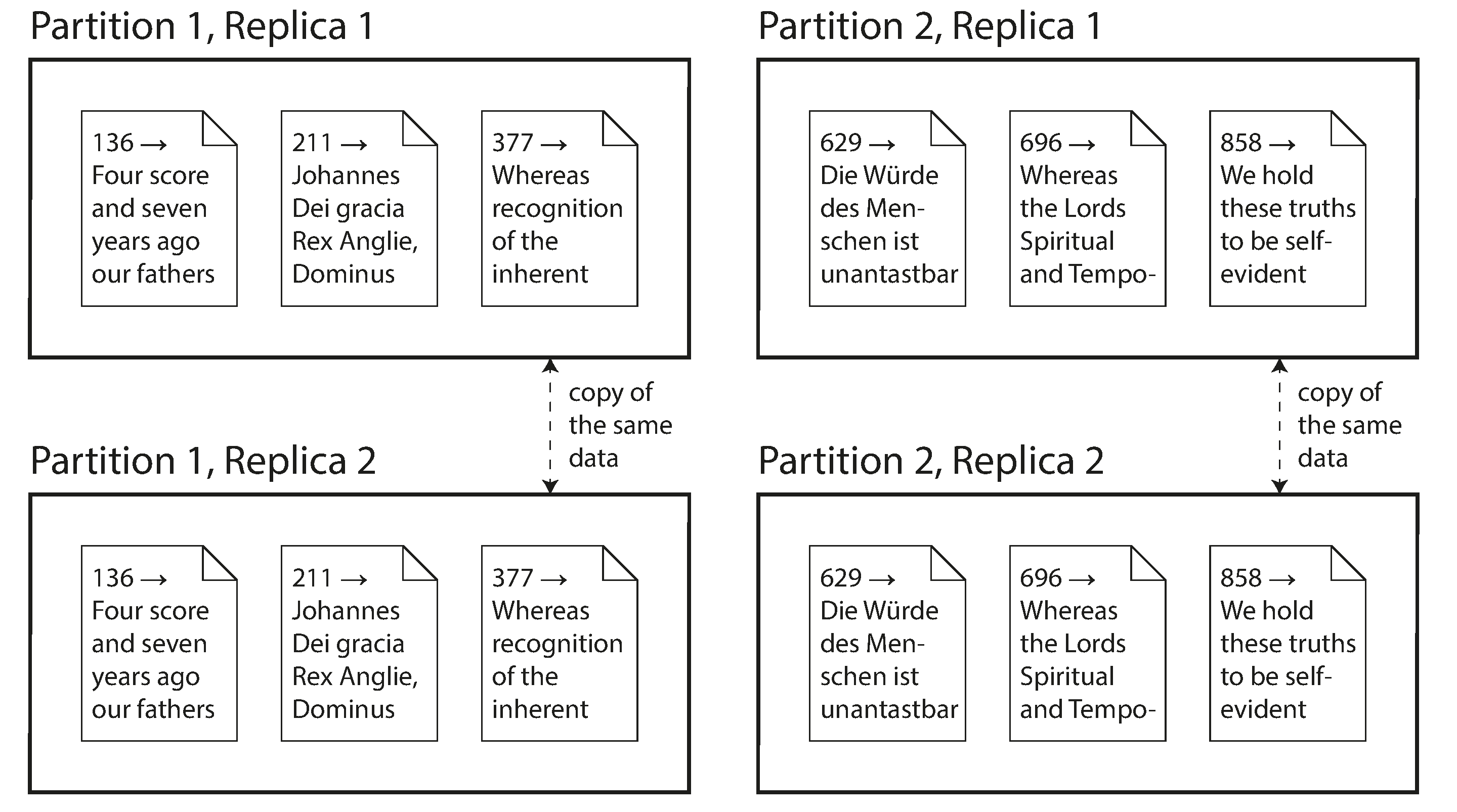
Figure II-1 A database split into two partitions, with two replicas per partition.

With an understanding of those concepts, we can discuss the difficult trade-offs that you need to make in a distributed system. We’ll discuss transactions in Chapter 8, as that will help you understand all the many things that can go wrong in a data system, and what you can do about them. We’ll conclude this part of the book by discussing the fundamental limitations of distributed systems in Chapters 9 and 10.

Later, in Part III of this book, we will discuss how you can take several (potentially distributed) datastores and integrate them into a larger system, satisfying the needs of a complex application. But first, let’s talk about distributed data.

6. Replication

7. Sharding

8. Transactions

9. The Trouble with Distributed Systems

10. Consistency and Consensus

References

Ulrich Drepper: “What Every Programmer Should Know About Memory,” akka‐dia.org, November 21, 2007. ↩︎ ↩︎
Ben Stopford: “Shared Nothing vs. Shared Disk Architectures: An Independent View,” benstopford.com, November 24, 2009. ↩︎
Michael Stonebraker: “The Case for Shared Nothing,” IEEE Database EngineeringBulletin, volume 9, number 1, pages 4–9, March 1986. ↩︎
Frank McSherry, Michael Isard, and Derek G. Murray: “Scalability! But at What COST?,” at 15th USENIX Workshop on Hot Topics in Operating Systems (HotOS),May 2015. ↩︎

6. Replication

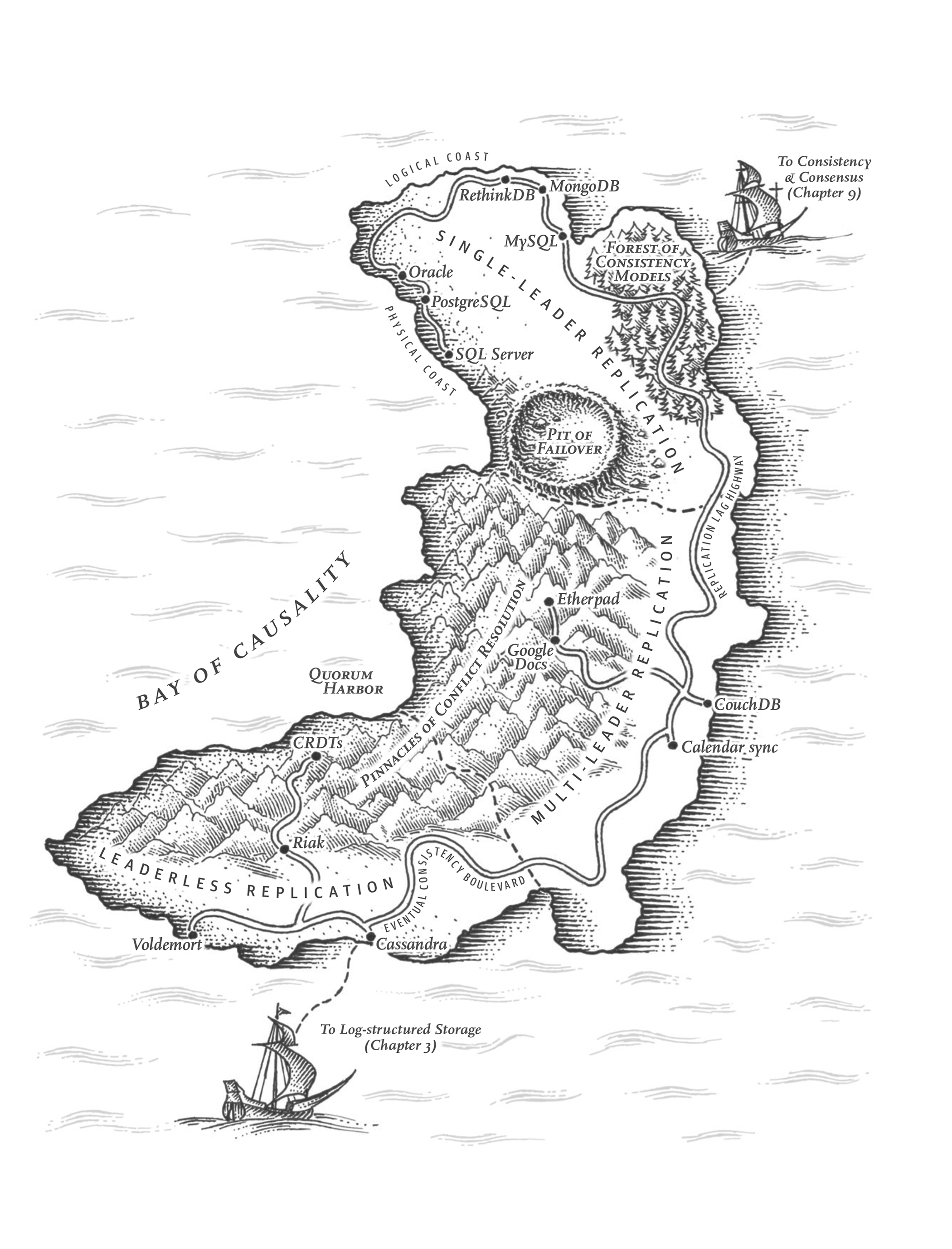
The major difference between a thing that might go wrong and a thing that cannot possibly go wrong is that when a thing that cannot possibly go wrong goes wrong it usually turns out to be impossible to get at or repair.

Douglas Adams, Mostly Harmless (1992)

Replication means keeping a copy of the same data on multiple machines that are connected via a network. As discussed in “Distributed versus Single-Node Systems”, there are several reasons why you might want to replicate data:

To keep data geographically close to your users (and thus reduce access latency)
To allow the system to continue working even if some of its parts have failed (and thus increase availability)
To scale out the number of machines that can serve read queries (and thus increase read throughput)

In this chapter we will assume that your dataset is small enough that each machine can hold a copy of the entire dataset. In Chapter 7 we will relax that assumption and discuss sharding (partitioning) of datasets that are too big for a single machine. In later chapters we will discuss various kinds of faults that can occur in a replicated data system, and how to deal with them.

If the data that you’re replicating does not change over time, then replication is easy: you just need to copy the data to every node once, and you’re done. All of the difficulty in replication lies in handling changes to replicated data, and that’s what this chapter is about. We will discuss three families of algorithms for replicating changes between nodes: single-leader, multi-leader, and leaderless replication. Almost all distributed databases use one of these three approaches. They all have various pros and cons, which we will examine in detail.

There are many trade-offs to consider with replication: for example, whether to use synchronous or asynchronous replication, and how to handle failed replicas. Those are often configuration options in databases, and although the details vary by database, the general principles are similar across many different implementations. We will discuss the consequences of such choices in this chapter.

Replication of databases is an old topic—the principles haven’t changed much since they were studied in the 1970s ¹, because the fundamental constraints of networks have remained the same. Despite being so old, concepts such as eventual consistency still cause confusion. In “Problems with Replication Lag” we will get more precise about eventual consistency and discuss things like the read-your-writes and monotonic reads guarantees.

BACKUPS AND REPLICATION

You might be wondering whether you still need backups if you have replication. The answer is yes, because they have different purposes: replicas quickly reflect writes from one node on other nodes, but backups store old snapshots of the data so that you can go back in time. If you accidentally delete some data, replication doesn’t help since the deletion will have also been propagated to the replicas, so you need a backup if you want to restore the deleted data.

In fact, replication and backups are often complementary to each other. Backups are sometimes part of the process of setting up replication, as we shall see in “Setting Up New Followers”. Conversely, archiving replication logs can be part of a backup process.

Some databases internally maintain immutable snapshots of past states, which serve as a kind of internal backup. However, this means keeping old versions of the data on the same storage media as the current state. If you have a large amount of data, it can be cheaper to keep the backups of old data in an object store that is optimized for infrequently-accessed data, and to store only the current state of the database in primary storage.

Single-Leader Replication

Each node that stores a copy of the database is called a replica. With multiple replicas, a question inevitably arises: how do we ensure that all the data ends up on all the replicas?

Every write to the database needs to be processed by every replica; otherwise, the replicas would no longer contain the same data. The most common solution is called leader-based replication, primary-backup, or active/passive. It works as follows (see Figure 6-1):

One of the replicas is designated the leader (also known as primary or source ²). When clients want to write to the database, they must send their requests to the leader, which first writes the new data to its local storage.
The other replicas are known as followers (read replicas, secondaries, or hot standbys). Whenever the leader writes new data to its local storage, it also sends the data change to all of its followers as part of a replication log or change stream. Each follower takes the log from the leader and updates its local copy of the database accordingly, by applying all writes in the same order as they were processed on the leader.
When a client wants to read from the database, it can query either the leader or any of the followers. However, writes are only accepted on the leader (the followers are read-only from the client’s point of view).

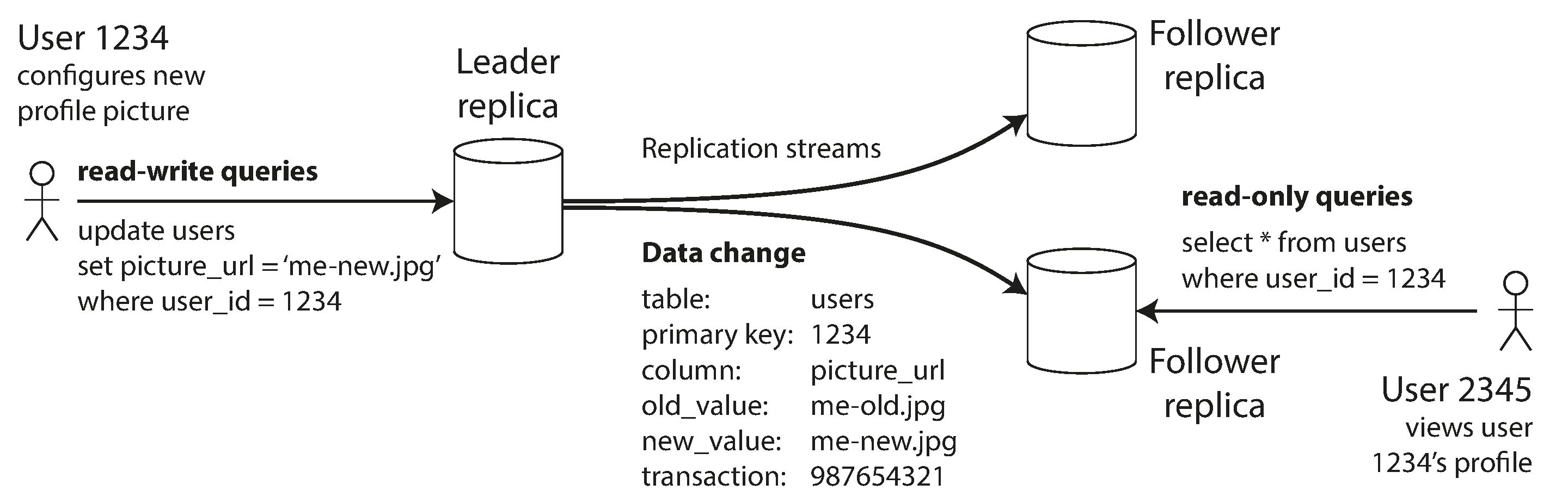
Figure 6-1 Single-leader replication directs all writes to a designated leader, which sends a stream of changes to the follower replicas.

If the database is sharded (see Chapter 7), each shard has one leader. Different shards may have their leaders on different nodes, but each shard must nevertheless have one leader node. In “Multi-Leader Replication” we will discuss an alternative model in which a system may have multiple leaders for the same shard at the same time.

Single-leader replication is very widely used. It’s a built-in feature of many relational databases, such as PostgreSQL, MySQL, Oracle Data Guard ³, and SQL Server’s Always On Availability Groups ⁴. It is also used in some document databases such as MongoDB and DynamoDB ⁵, message brokers such as Kafka, replicated block devices such as DRBD, and some network filesystems. Many consensus algorithms such as Raft, which is used for replication in CockroachDB ⁶, TiDB ⁷, etcd, and RabbitMQ quorum queues (among others), are also based on a single leader, and automatically elect a new leader if the old one fails (we will discuss consensus in more detail in Chapter 10).

Note

In older documents you may see the term master–slave replication. It means the same as leader-based replication, but the term should be avoided as it is widely considered offensive ⁸.

Synchronous Versus Asynchronous Replication

An important detail of a replicated system is whether the replication happens synchronously or asynchronously. (In relational databases, this is often a configurable option; other systems are often hardcoded to be either one or the other.)

Think about what happens in Figure 6-1, where the user of a website updates their profile image. At some point in time, the client sends the update request to the leader; shortly afterward, it is received by the leader. At some point, the leader forwards the data change to the followers. Eventually, the leader notifies the client that the update was successful. Figure 6-2 shows one possible way how the timings could work out.

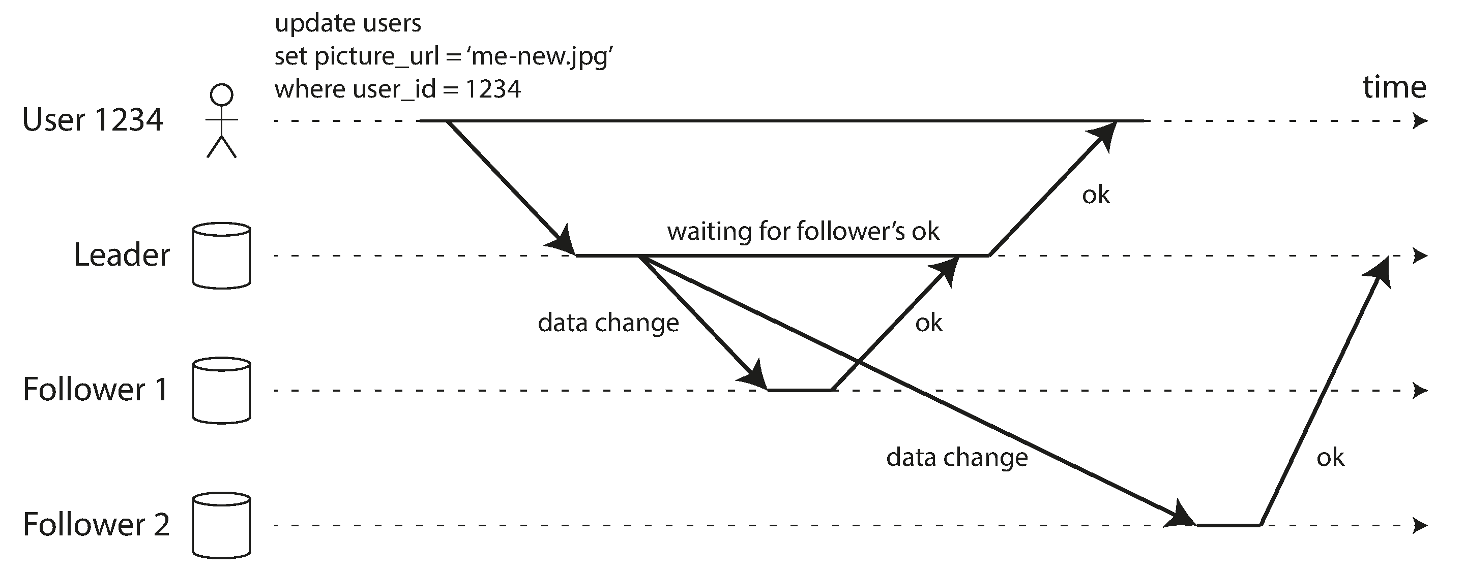
Figure 6-2 Leader-based replication with one synchronous and one asynchronous follower.

In the example of Figure 6-2, the replication to follower 1 is synchronous: the leader waits until follower 1 has confirmed that it received the write before reporting success to the user, and before making the write visible to other clients. The replication to follower 2 is asynchronous: the leader sends the message, but doesn’t wait for a response from the follower.

The diagram shows that there is a substantial delay before follower 2 processes the message. Normally, replication is quite fast: most database systems apply changes to followers in less than a second. However, there is no guarantee of how long it might take. There are circumstances when followers might fall behind the leader by several minutes or more; for example, if a follower is recovering from a failure, if the system is operating near maximum capacity, or if there are network problems between the nodes.

The advantage of synchronous replication is that the follower is guaranteed to have an up-to-date copy of the data that is consistent with the leader. If the leader suddenly fails, we can be sure that the data is still available on the follower. The disadvantage is that if the synchronous follower doesn’t respond (because it has crashed, or there is a network fault, or for any other reason), the write cannot be processed. The leader must block all writes and wait until the synchronous replica is available again.

For that reason, it is impracticable for all followers to be synchronous: any one node outage would cause the whole system to grind to a halt. In practice, if a database offers synchronous replication, it often means that one of the followers is synchronous, and the others are asynchronous. If the synchronous follower becomes unavailable or slow, one of the asynchronous followers is made synchronous. This guarantees that you have an up-to-date copy of the data on at least two nodes: the leader and one synchronous follower. This configuration is sometimes also called semi-synchronous.

In some systems, a majority (e.g., 3 out of 5 replicas, including the leader) of replicas is updated synchronously, and the remaining minority is asynchronous. This is an example of a quorum, which we will discuss further in “Quorums for reading and writing”. Majority quorums are often used in systems that use a consensus protocol for automatic leader election, which we will return to in Chapter 10.

Sometimes, leader-based replication is configured to be completely asynchronous. In this case, if the leader fails and is not recoverable, any writes that have not yet been replicated to followers are lost. This means that a write is not guaranteed to be durable, even if it has been confirmed to the client. However, a fully asynchronous configuration has the advantage that the leader can continue processing writes, even if all of its followers have fallen behind.

Weakening durability may sound like a bad trade-off, but asynchronous replication is nevertheless widely used, especially if there are many followers or if they are geographically distributed ⁹. We will return to this issue in “Problems with Replication Lag”.

Setting Up New Followers

From time to time, you need to set up new followers—perhaps to increase the number of replicas, or to replace failed nodes. How do you ensure that the new follower has an accurate copy of the leader’s data?

Simply copying data files from one node to another is typically not sufficient: clients are constantly writing to the database, and the data is always in flux, so a standard file copy would see different parts of the database at different points in time. The result might not make any sense.

You could make the files on disk consistent by locking the database (making it unavailable for writes), but that would go against our goal of high availability. Fortunately, setting up a follower can usually be done without downtime. Conceptually, the process looks like this:

Take a consistent snapshot of the leader’s database at some point in time—if possible, without taking a lock on the entire database. Most databases have this feature, as it is also required for backups. In some cases, third-party tools are needed, such as Percona XtraBackup for MySQL.
Copy the snapshot to the new follower node.
The follower connects to the leader and requests all the data changes that have happened since the snapshot was taken. This requires that the snapshot is associated with an exact position in the leader’s replication log. That position has various names: for example, PostgreSQL calls it the log sequence number; MySQL has two mechanisms, binlog coordinates and global transaction identifiers (GTIDs).
When the follower has processed the backlog of data changes since the snapshot, we say it has caught up. It can now continue to process data changes from the leader as they happen.

The practical steps of setting up a follower vary significantly by database. In some systems the process is fully automated, whereas in others it can be a somewhat arcane multi-step workflow that needs to be manually performed by an administrator.

You can also archive the replication log to an object store; along with periodic snapshots of the whole database in the object store this is a good way of implementing database backups and disaster recovery. You can also perform steps 1 and 2 of setting up a new follower by downloading those files from the object store. For example, WAL-G does this for PostgreSQL, MySQL, and SQL Server, and Litestream does the equivalent for SQLite.

DATABASES BACKED BY OBJECT STORAGE

Object storage can be used for more than archiving data. Many databases are beginning to use object stores such as Amazon Web Services S3, Google Cloud Storage, and Azure Blob Storage to serve data for live queries. Storing database data in object storage has many benefits:

Object storage is inexpensive compared to other cloud storage options, which allow cloud databases to store less-often queried data on cheaper, higher-latency storage while serving the working set from memory, SSDs, and NVMe.
Object stores also provide multi-zone, dual-region, or multi-region replication with very high durability guarantees. This also allows databases to bypass inter-zone network fees.
Databases can use an object store’s conditional write feature—essentially, a compare-and-set (CAS) operation—to implement transactions and leadership election ¹⁰ ¹¹
Storing data from multiple databases in the same object store can simplify data integration, particularly when open formats such as Apache Parquet and Apache Iceberg are used.

These benefits dramatically simplify the database architecture by shifting the responsibility of transactions, leadership election, and replication to object storage.

Systems that adopt object storage for replication must grapple with some tradeoffs. Notably, object stores have much higher read and write latencies than local disks or virtual block devices such as EBS. Many cloud providers also charge a per-API call fee, which forces systems to batch reads and writes to reduce cost. Such batching further increases latency. Moreover, many object stores do not offer standard filesystem interfaces. This prevents systems that lack object storage integration from leveraging object storage. Interfaces such as filesystem in userspace (FUSE) allow operators to mount object store buckets as filesystems that applications can use without knowing their data is stored on object storage. Still, many FUSE interfaces to object stores lack POSIX features such as non-sequential writes or symlinks, which systems might depend on.

Different systems deal with these trade-offs in various ways. Some introduce a tiered storage architecture that places less frequently accessed data on object storage while new or frequently accessed data is kept on faster storage devices such as SSDs, NVMe, or even in memory. Other systems use object storage as their primary storage tier, but use a separate low-latency storage system such as Amazon’s EBS or Neon’s Safekeepers ¹²) to store their WAL. Recently, some systems have gone even farther by adopting a zero-disk architecture (ZDA). ZDA-based systems persist all data to object storage and use disks and memory strictly for caching. This allows nodes to have no persistent state, which dramatically simplifies operations. WarpStream, Confluent Freight, Buf’s Bufstream, and Redpanda Serverless are all Kafka-compatible systems built using a zero-disk architecture. Nearly every modern cloud data warehouse also adopts such an architecture, as does Turbopuffer (a vector search engine), and SlateDB (a cloud-native LSM storage engine).

Handling Node Outages

Any node in the system can go down, perhaps unexpectedly due to a fault, but just as likely due to planned maintenance (for example, rebooting a machine to install a kernel security patch). Being able to reboot individual nodes without downtime is a big advantage for operations and maintenance. Thus, our goal is to keep the system as a whole running despite individual node failures, and to keep the impact of a node outage as small as possible.

How do you achieve high availability with leader-based replication?

Follower failure: Catch-up recovery

On its local disk, each follower keeps a log of the data changes it has received from the leader. If a follower crashes and is restarted, or if the network between the leader and the follower is temporarily interrupted, the follower can recover quite easily: from its log, it knows the last transaction that was processed before the fault occurred. Thus, the follower can connect to the leader and request all the data changes that occurred during the time when the follower was disconnected. When it has applied these changes, it has caught up to the leader and can continue receiving a stream of data changes as before.

Although follower recovery is conceptually simple, it can be challenging in terms of performance: if the database has a high write throughput or if the follower has been offline for a long time, there might be a lot of writes to catch up on. There will be high load on both the recovering follower and the leader (which needs to send the backlog of writes to the follower) while this catch-up is ongoing.

The leader can delete its log of writes once all followers have confirmed that they have processed it, but if a follower is unavailable for a long time, the leader faces a choice: either it retains the log until the follower recovers and catches up (at the risk of running out of disk space on the leader), or it deletes the log that the unavailable follower has not yet acknowledged (in which case the follower won’t be able to recover from the log, and will have to be restored from a backup when it comes back).

Leader failure: Failover

Handling a failure of the leader is trickier: one of the followers needs to be promoted to be the new leader, clients need to be reconfigured to send their writes to the new leader, and the other followers need to start consuming data changes from the new leader. This process is called failover.

Failover can happen manually (an administrator is notified that the leader has failed and takes the necessary steps to make a new leader) or automatically. An automatic failover process usually consists of the following steps:

Determining that the leader has failed. There are many things that could potentially go wrong: crashes, power outages, network issues, and more. There is no foolproof way of detecting what has gone wrong, so most systems simply use a timeout: nodes frequently bounce messages back and forth between each other, and if a node doesn’t respond for some period of time—say, 30 seconds—it is assumed to be dead. (If the leader is deliberately taken down for planned maintenance, this doesn’t apply.)
Choosing a new leader. This could be done through an election process (where the leader is chosen by a majority of the remaining replicas), or a new leader could be appointed by a previously established controller node ¹³. The best candidate for leadership is usually the replica with the most up-to-date data changes from the old leader (to minimize any data loss). Getting all the nodes to agree on a new leader is a consensus problem, discussed in detail in Chapter 10.
Reconfiguring the system to use the new leader. Clients now need to send their write requests to the new leader (we discuss this in “Request Routing”). If the old leader comes back, it might still believe that it is the leader, not realizing that the other replicas have forced it to step down. The system needs to ensure that the old leader becomes a follower and recognizes the new leader.

Failover is fraught with things that can go wrong:

If asynchronous replication is used, the new leader may not have received all the writes from the old leader before it failed. If the former leader rejoins the cluster after a new leader has been chosen, what should happen to those writes? The new leader may have received conflicting writes in the meantime. The most common solution is for the old leader’s unreplicated writes to simply be discarded, which means that writes you believed to be committed actually weren’t durable after all.
Discarding writes is especially dangerous if other storage systems outside of the database need to be coordinated with the database contents. For example, in one incident at GitHub ¹⁴, an out-of-date MySQL follower was promoted to leader. The database used an autoincrementing counter to assign primary keys to new rows, but because the new leader’s counter lagged behind the old leader’s, it reused some primary keys that were previously assigned by the old leader. These primary keys were also used in a Redis store, so the reuse of primary keys resulted in inconsistency between MySQL and Redis, which caused some private data to be disclosed to the wrong users.
In certain fault scenarios (see Chapter 9), it could happen that two nodes both believe that they are the leader. This situation is called split brain, and it is dangerous: if both leaders accept writes, and there is no process for resolving conflicts (see “Multi-Leader Replication”), data is likely to be lost or corrupted. As a safety catch, some systems have a mechanism to shut down one node if two leaders are detected. However, if this mechanism is not carefully designed, you can end up with both nodes being shut down ¹⁵. Moreover, there is a risk that by the time the split brain is detected and the old node is shut down, it is already too late and data has already been corrupted.
What is the right timeout before the leader is declared dead? A longer timeout means a longer time to recovery in the case where the leader fails. However, if the timeout is too short, there could be unnecessary failovers. For example, a temporary load spike could cause a node’s response time to increase above the timeout, or a network glitch could cause delayed packets. If the system is already struggling with high load or network problems, an unnecessary failover is likely to make the situation worse, not better.

Note

Guarding against split brain by limiting or shutting down old leaders is known as fencing or, more emphatically, Shoot The Other Node In The Head (STONITH). We will discuss fencing in more detail in “Distributed Locks and Leases”.

There are no easy solutions to these problems. For this reason, some operations teams prefer to perform failovers manually, even if the software supports automatic failover.

The most important thing with failover is to pick an up-to-date follower as the new leader—if synchronous or semi-synchronous replication is used, this would be the follower that the old leader waited for before acknowledging writes. With asynchronous replication, you can pick the follower with the greatest log sequence number. This minimizes the amount of data that is lost during failover: losing a fraction of a second of writes may be tolerable, but picking a follower that is behind by several days could be catastrophic.

These issues—node failures; unreliable networks; and trade-offs around replica consistency, durability, availability, and latency—are in fact fundamental problems in distributed systems. In Chapter 9 and Chapter 10 we will discuss them in greater depth.

Implementation of Replication Logs

How does leader-based replication work under the hood? Several different replication methods are used in practice, so let’s look at each one briefly.

Statement-based replication

In the simplest case, the leader logs every write request (statement) that it executes and sends that statement log to its followers. For a relational database, this means that every INSERT, UPDATE, or DELETE statement is forwarded to followers, and each follower parses and executes that SQL statement as if it had been received from a client.

Although this may sound reasonable, there are various ways in which this approach to replication can break down:

Any statement that calls a nondeterministic function, such as NOW() to get the current date and time or RAND() to get a random number, is likely to generate a different value on each replica.
If statements use an autoincrementing column, or if they depend on the existing data in the database (e.g., UPDATE … WHERE <some condition>), they must be executed in exactly the same order on each replica, or else they may have a different effect. This can be limiting when there are multiple concurrently executing transactions.
Statements that have side effects (e.g., triggers, stored procedures, user-defined functions) may result in different side effects occurring on each replica, unless the side effects are absolutely deterministic.

It is possible to work around those issues—for example, the leader can replace any nondeterministic function calls with a fixed return value when the statement is logged so that the followers all get the same value. The idea of executing deterministic statements in a fixed order is similar to the event sourcing model that we previously discussed in “Event Sourcing and CQRS”. This approach is also known as state machine replication, and we will discuss the theory behind it in “Using shared logs”.

Statement-based replication was used in MySQL before version 5.1. It is still sometimes used today, as it is quite compact, but by default MySQL now switches to row-based replication (discussed shortly) if there is any nondeterminism in a statement. VoltDB uses statement-based replication, and makes it safe by requiring transactions to be deterministic ¹⁶. However, determinism can be hard to guarantee in practice, so many databases prefer other replication methods.

Write-ahead log (WAL) shipping

In Chapter 4 we saw that a write-ahead log is needed to make B-tree storage engines robust: every modification is first written to the WAL so that the tree can be restored to a consistent state after a crash. Since the WAL contains all the information necessary to restore the indexes and heap into a consistent state, we can use the exact same log to build a replica on another node: besides writing the log to disk, the leader also sends it across the network to its followers. When the follower processes this log, it builds a copy of the exact same files as found on the leader.

This method of replication is used in PostgreSQL and Oracle, among others ¹⁷ ¹⁸ The main disadvantage is that the log describes the data on a very low level: a WAL contains details of which bytes were changed in which disk blocks. This makes replication tightly coupled to the storage engine. If the database changes its storage format from one version to another, it is typically not possible to run different versions of the database software on the leader and the followers.

That may seem like a minor implementation detail, but it can have a big operational impact. If the replication protocol allows the follower to use a newer software version than the leader, you can perform a zero-downtime upgrade of the database software by first upgrading the followers and then performing a failover to make one of the upgraded nodes the new leader. If the replication protocol does not allow this version mismatch, as is often the case with WAL shipping, such upgrades require downtime.

Logical (row-based) log replication

An alternative is to use different log formats for replication and for the storage engine, which allows the replication log to be decoupled from the storage engine internals. This kind of replication log is called a logical log, to distinguish it from the storage engine’s (physical) data representation.

A logical log for a relational database is usually a sequence of records describing writes to database tables at the granularity of a row:

For an inserted row, the log contains the new values of all columns.
For a deleted row, the log contains enough information to uniquely identify the row that was deleted. Typically this would be the primary key, but if there is no primary key on the table, the old values of all columns need to be logged.
For an updated row, the log contains enough information to uniquely identify the updated row, and the new values of all columns (or at least the new values of all columns that changed).

A transaction that modifies several rows generates several such log records, followed by a record indicating that the transaction was committed. MySQL keeps a separate logical replication log, called the binlog, in addition to the WAL (when configured to use row-based replication). PostgreSQL implements logical replication by decoding the physical WAL into row insertion/update/delete events ¹⁹.

Since a logical log is decoupled from the storage engine internals, it can more easily be kept backward compatible, allowing the leader and the follower to run different versions of the database software. This in turn enables upgrading to a new version with minimal downtime ²⁰.

A logical log format is also easier for external applications to parse. This aspect is useful if you want to send the contents of a database to an external system, such as a data warehouse for offline analysis, or for building custom indexes and caches ²¹. This technique is called change data capture, and we will return to it in “Change Data Capture”.

Problems with Replication Lag

Being able to tolerate node failures is just one reason for wanting replication. As mentioned in “Distributed versus Single-Node Systems”, other reasons are scalability (processing more requests than a single machine can handle) and latency (placing replicas geographically closer to users).

Leader-based replication requires all writes to go through a single node, but read-only queries can go to any replica. For workloads that consist of mostly reads and only a small percentage of writes (which is often the case with online services), there is an attractive option: create many followers, and distribute the read requests across those followers. This removes load from the leader and allows read requests to be served by nearby replicas.

In this read-scaling architecture, you can increase the capacity for serving read-only requests simply by adding more followers. However, this approach only realistically works with asynchronous replication—if you tried to synchronously replicate to all followers, a single node failure or network outage would make the entire system unavailable for writing. And the more nodes you have, the likelier it is that one will be down, so a fully synchronous configuration would be very unreliable.

Unfortunately, if an application reads from an asynchronous follower, it may see outdated information if the follower has fallen behind. This leads to apparent inconsistencies in the database: if you run the same query on the leader and a follower at the same time, you may get different results, because not all writes have been reflected in the follower. This inconsistency is just a temporary state—if you stop writing to the database and wait a while, the followers will eventually catch up and become consistent with the leader. For that reason, this effect is known as eventual consistency ²².

Note

The term eventual consistency was coined by Douglas Terry et al. ²³, popularized by Werner Vogels ²⁴, and became the battle cry of many NoSQL projects. However, not only NoSQL databases are eventually consistent: followers in an asynchronously replicated relational database have the same characteristics.

The term “eventually” is deliberately vague: in general, there is no limit to how far a replica can fall behind. In normal operation, the delay between a write happening on the leader and being reflected on a follower—the replication lag—may be only a fraction of a second, and not noticeable in practice. However, if the system is operating near capacity or if there is a problem in the network, the lag can easily increase to several seconds or even minutes.

When the lag is so large, the inconsistencies it introduces are not just a theoretical issue but a real problem for applications. In this section we will highlight three examples of problems that are likely to occur when there is replication lag. We’ll also outline some approaches to solving them.

Reading Your Own Writes

Many applications let the user submit some data and then view what they have submitted. This might be a record in a customer database, or a comment on a discussion thread, or something else of that sort. When new data is submitted, it must be sent to the leader, but when the user views the data, it can be read from a follower. This is especially appropriate if data is frequently viewed but only occasionally written.

With asynchronous replication, there is a problem, illustrated in Figure 6-3: if the user views the data shortly after making a write, the new data may not yet have reached the replica. To the user, it looks as though the data they submitted was lost, so they will be understandably unhappy.

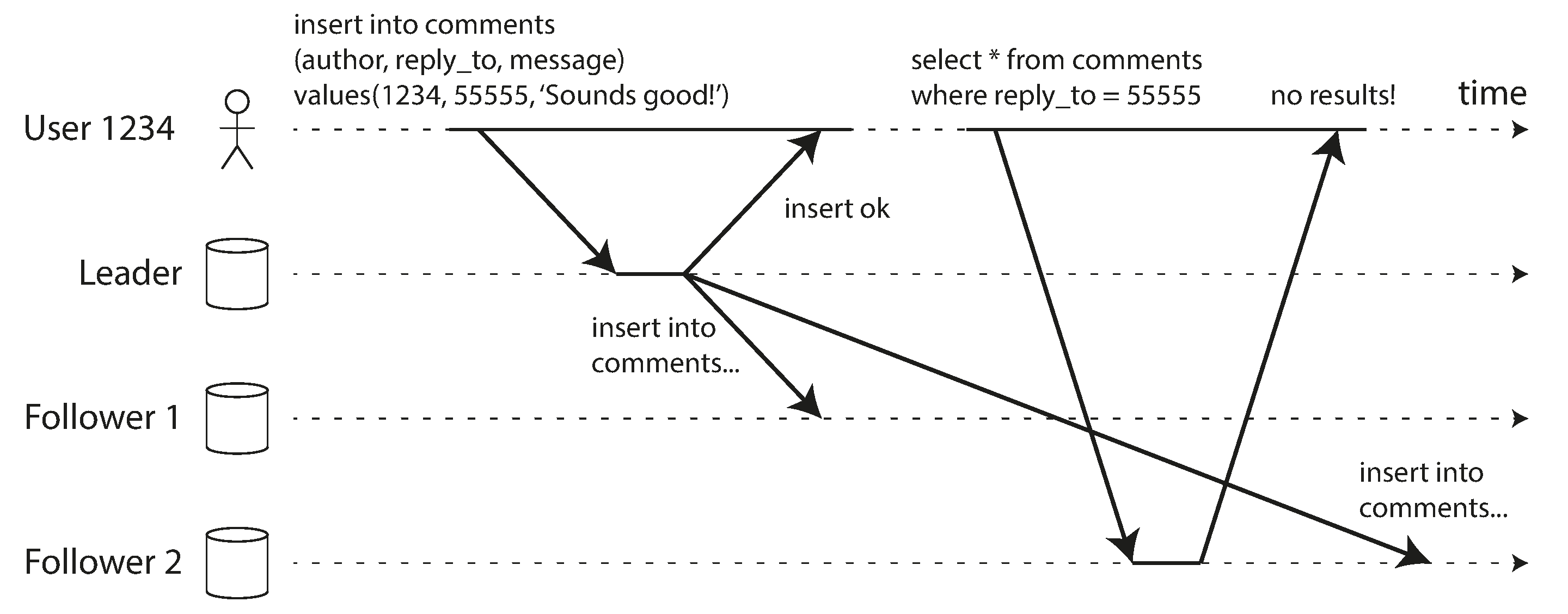
Figure 6-3 A user makes a write, followed by a read from a stale replica. To prevent this anomaly, we need read-after-write consistency.

In this situation, we need read-after-write consistency, also known as read-your-writes consistency ²³. This is a guarantee that if the user reloads the page, they will always see any updates they submitted themselves. It makes no promises about other users: other users’ updates may not be visible until some later time. However, it reassures the user that their own input has been saved correctly.

How can we implement read-after-write consistency in a system with leader-based replication? There are various possible techniques. To mention a few:

When reading something that the user may have modified, read it from the leader or a synchronously updated follower; otherwise, read it from an asynchronously updated follower. This requires that you have some way of knowing whether something might have been modified, without actually querying it. For example, user profile information on a social network is normally only editable by the owner of the profile, not by anybody else. Thus, a simple rule is: always read the user’s own profile from the leader, and any other users’ profiles from a follower.
If most things in the application are potentially editable by the user, that approach won’t be effective, as most things would have to be read from the leader (negating the benefit of read scaling). In that case, other criteria may be used to decide whether to read from the leader. For example, you could track the time of the last update and, for one minute after the last update, make all reads from the leader ²⁵. You could also monitor the replication lag on followers and prevent queries on any follower that is more than one minute behind the leader.
The client can remember the timestamp of its most recent write—then the system can ensure that the replica serving any reads for that user reflects updates at least until that timestamp. If a replica is not sufficiently up to date, either the read can be handled by another replica or the query can wait until the replica has caught up ²⁶. The timestamp could be a logical timestamp (something that indicates ordering of writes, such as the log sequence number) or the actual system clock (in which case clock synchronization becomes critical; see “Unreliable Clocks”).
If your replicas are distributed across regions (for geographical proximity to users or for availability), there is additional complexity. Any request that needs to be served by the leader must be routed to the region that contains the leader.

Another complication arises when the same user is accessing your service from multiple devices, for example a desktop web browser and a mobile app. In this case you may want to provide cross-device read-after-write consistency: if the user enters some information on one device and then views it on another device, they should see the information they just entered.

In this case, there are some additional issues to consider:

Approaches that require remembering the timestamp of the user’s last update become more difficult, because the code running on one device doesn’t know what updates have happened on the other device. This metadata will need to be centralized.
If your replicas are distributed across different regions, there is no guarantee that connections from different devices will be routed to the same region. (For example, if the user’s desktop computer uses the home broadband connection and their mobile device uses the cellular data network, the devices’ network routes may be completely different.) If your approach requires reading from the leader, you may first need to route requests from all of a user’s devices to the same region.

![TIP] Regions and Availability Zones

We use the term region to refer to one or more datacenters in a single geographic location. Cloud providers locate multiple datacenters in the same geographic region. Each datacenter is referred to as an availability zone or simply zone. Thus, a single cloud region is made up of multiple zones. Each zone is a separate datacenter located in separate physical facility with its own power, cooling, and so on.

Zones in the same region are connected by very high speed network connections. Latency is low enough that most distributed systems can run with nodes spread across multiple zones in the same region as though they were in a single zone. Multi-zone configurations allow distributed systems to survive zonal outages where one zone goes offline, but they do not protect against regional outages where all zones in a region are unavailable. To survive a regional outage, a distributed system must be deployed across multiple regions, which can result in higher latencies, lower throughput, and increased cloud networking bills. We will discuss these tradeoffs more in “Multi-leader replication topologies”. For now, just know that when we say region, we mean a collection of zones/datacenters in a single geographic location.

Monotonic Reads

Our second example of an anomaly that can occur when reading from asynchronous followers is that it’s possible for a user to see things moving backward in time.

This can happen if a user makes several reads from different replicas. For example, Figure 6-4 shows user 2345 making the same query twice, first to a follower with little lag, then to a follower with greater lag. (This scenario is quite likely if the user refreshes a web page, and each request is routed to a random server.) The first query returns a comment that was recently added by user 1234, but the second query doesn’t return anything because the lagging follower has not yet picked up that write. In effect, the second query observes the system state at an earlier point in time than the first query. This wouldn’t be so bad if the first query hadn’t returned anything, because user 2345 probably wouldn’t know that user 1234 had recently added a comment. However, it’s very confusing for user 2345 if they first see user 1234’s comment appear, and then see it disappear again.

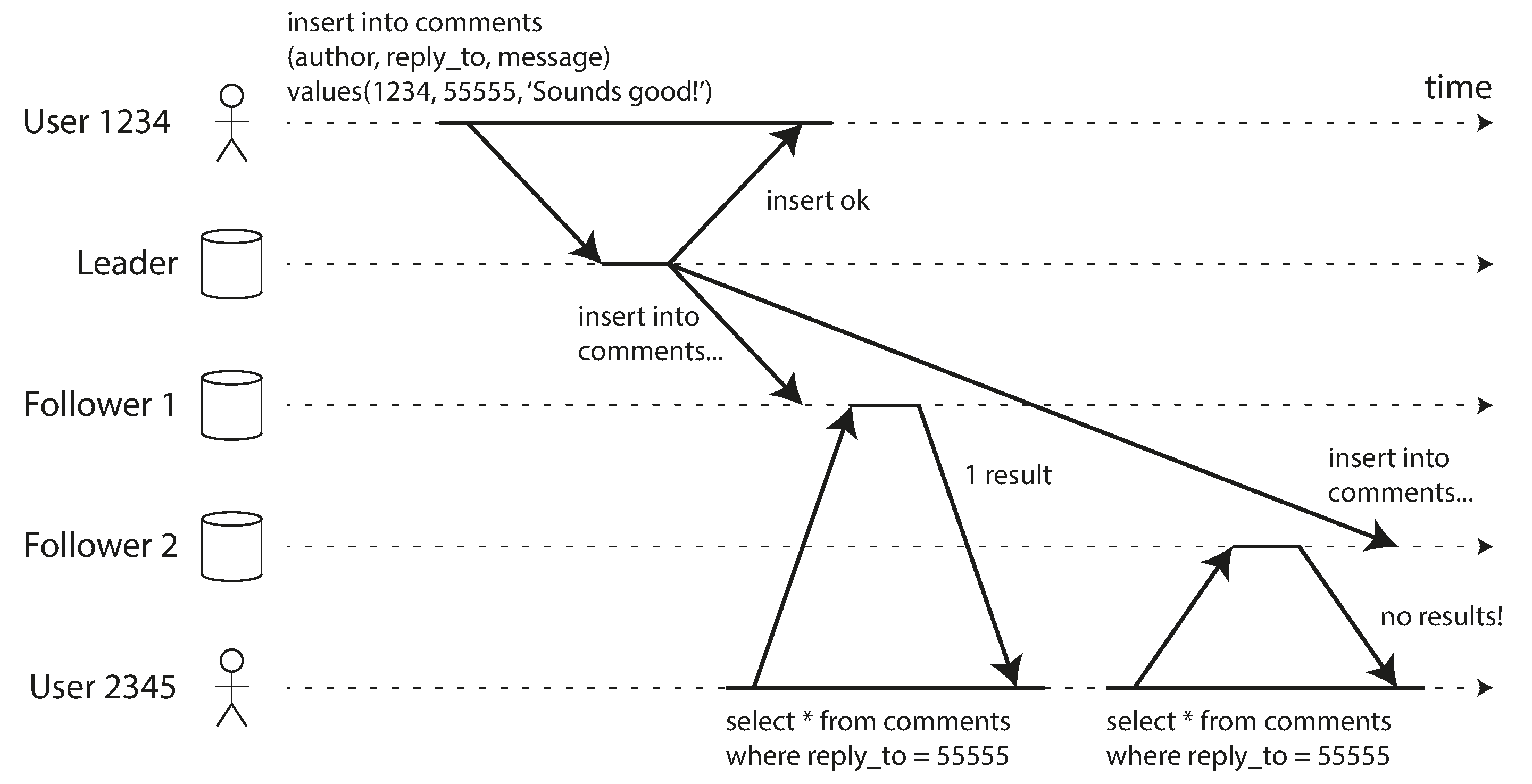
Figure 6-4 A user first reads from a fresh replica, then from a stale replica. Time appears to go backward. To prevent this anomaly, we need monotonic reads.

Monotonic reads ²² is a guarantee that this kind of anomaly does not happen. It’s a lesser guarantee than strong consistency, but a stronger guarantee than eventual consistency. When you read data, you may see an old value; monotonic reads only means that if one user makes several reads in sequence, they will not see time go backward—i.e., they will not read older data after having previously read newer data.

One way of achieving monotonic reads is to make sure that each user always makes their reads from the same replica (different users can read from different replicas). For example, the replica can be chosen based on a hash of the user ID, rather than randomly. However, if that replica fails, the user’s queries will need to be rerouted to another replica.

Consistent Prefix Reads

Our third example of replication lag anomalies concerns violation of causality. Imagine the following short dialog between Mr. Poons and Mrs. Cake:

Mr. Poons: How far into the future can you see, Mrs. Cake?
Mrs. Cake: About ten seconds usually, Mr. Poons.

There is a causal dependency between those two sentences: Mrs. Cake heard Mr. Poons’s question and answered it.

Now, imagine a third person is listening to this conversation through followers. The things said by Mrs. Cake go through a follower with little lag, but the things said by Mr. Poons have a longer replication lag (see Figure 6-5). This observer would hear the following:

Mrs. Cake: About ten seconds usually, Mr. Poons.
Mr. Poons: How far into the future can you see, Mrs. Cake?

To the observer it looks as though Mrs. Cake is answering the question before Mr. Poons has even asked it. Such psychic powers are impressive, but very confusing ²⁷.

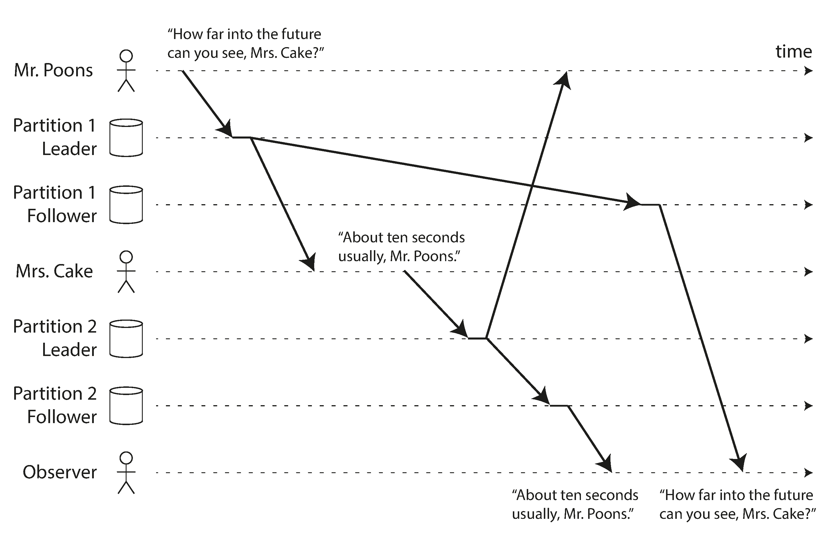
Figure 6-5 If some shards are replicated slower than others, an observer may see the answer before they see the question.

Preventing this kind of anomaly requires another type of guarantee: consistent prefix reads ²². This guarantee says that if a sequence of writes happens in a certain order, then anyone reading those writes will see them appear in the same order.

This is a particular problem in sharded (partitioned) databases, which we will discuss in Chapter 7. If the database always applies writes in the same order, reads always see a consistent prefix, so this anomaly cannot happen. However, in many distributed databases, different shards operate independently, so there is no global ordering of writes: when a user reads from the database, they may see some parts of the database in an older state and some in a newer state.

One solution is to make sure that any writes that are causally related to each other are written to the same shard—but in some applications that cannot be done efficiently. There are also algorithms that explicitly keep track of causal dependencies, a topic that we will return to in “The “happens-before” relation and concurrency”.

Solutions for Replication Lag

When working with an eventually consistent system, it is worth thinking about how the application behaves if the replication lag increases to several minutes or even hours. If the answer is “no problem,” that’s great. However, if the result is a bad experience for users, it’s important to design the system to provide a stronger guarantee, such as read-after-write. Pretending that replication is synchronous when in fact it is asynchronous is a recipe for problems down the line.

As discussed earlier, there are ways in which an application can provide a stronger guarantee than the underlying database—for example, by performing certain kinds of reads on the leader or a synchronously updated follower. However, dealing with these issues in application code is complex and easy to get wrong.

The simplest programming model for application developers is to choose a database that provides a strong consistency guarantee for replicas such as linearizability (see Chapter 10), and ACID transactions (see Chapter 8). This allows you to mostly ignore the challenges that arise from replication, and treat the database as if it had just a single node. In the early 2010s the NoSQL movement promoted the view that these features limited scalability, and that large-scale systems would have to embrace eventual consistency.

However, since then, a number of databases started providing strong consistency and transactions while also offering the fault tolerance, high availability, and scalability advantages of a distributed database. As mentioned in “Relational Model versus Document Model”, this trend is known as NewSQL to contrast with NoSQL (although it’s less about SQL specifically, and more about new approaches to scalable transaction management).

Even though scalable, strongly consistent distributed databases are now available, there are still good reasons why some applications choose to use different forms of replication that offer weaker consistency guarantees: they can offer stronger resilience in the face of network interruptions, and have lower overheads compared to transactional systems. We will explore such approaches in the rest of this chapter.

Multi-Leader Replication

So far in this chapter we have only considered replication architectures using a single leader. Although that is a common approach, there are interesting alternatives.

Single-leader replication has one major downside: all writes must go through the one leader. If you can’t connect to the leader for any reason, for example due to a network interruption between you and the leader, you can’t write to the database.

A natural extension of the single-leader replication model is to allow more than one node to accept writes. Replication still happens in the same way: each node that processes a write must forward that data change to all the other nodes. We call this a multi-leader configuration (also known as active/active or bidirectional replication). In this setup, each leader simultaneously acts as a follower to the other leaders.

As with single-leader replication, there is a choice between making it synchronous or asynchronous. Let’s say you have two leaders, A and B, and you’re trying to write to A. If writes are synchronously replicated from A to B, and the network between the two nodes is interrupted, you can’t write to A until the network comes back. Synchronous multi-leader replication thus gives you a model that is very similar to single-leader replication, i.e. if you had made B the leader and A simply forwards any write requests to B to be executed.

For that reason, we won’t go further into synchronous multi-leader replication, and simply treat it as equivalent to single-leader replication. The rest of this section focusses on asynchronous multi-leader replication, in which any leader can process writes even when its connection to the other leaders is interrupted.

Geographically Distributed Operation

It rarely makes sense to use a multi-leader setup within a single region, because the benefits rarely outweigh the added complexity. However, there are some situations in which this configuration is reasonable.

Imagine you have a database with replicas in several different regions (perhaps so that you can tolerate the failure of an entire region, or perhaps in order to be closer to your users). This is known as a geographically distributed, geo-distributed or geo-replicated setup. With single-leader replication, the leader has to be in one of the regions, and all writes must go through that region.

In a multi-leader configuration, you can have a leader in each region. Figure 6-6 shows what this architecture might look like. Within each region, regular leader–follower replication is used (with followers maybe in a different availability zone from the leader); between regions, each region’s leader replicates its changes to the leaders in other regions.

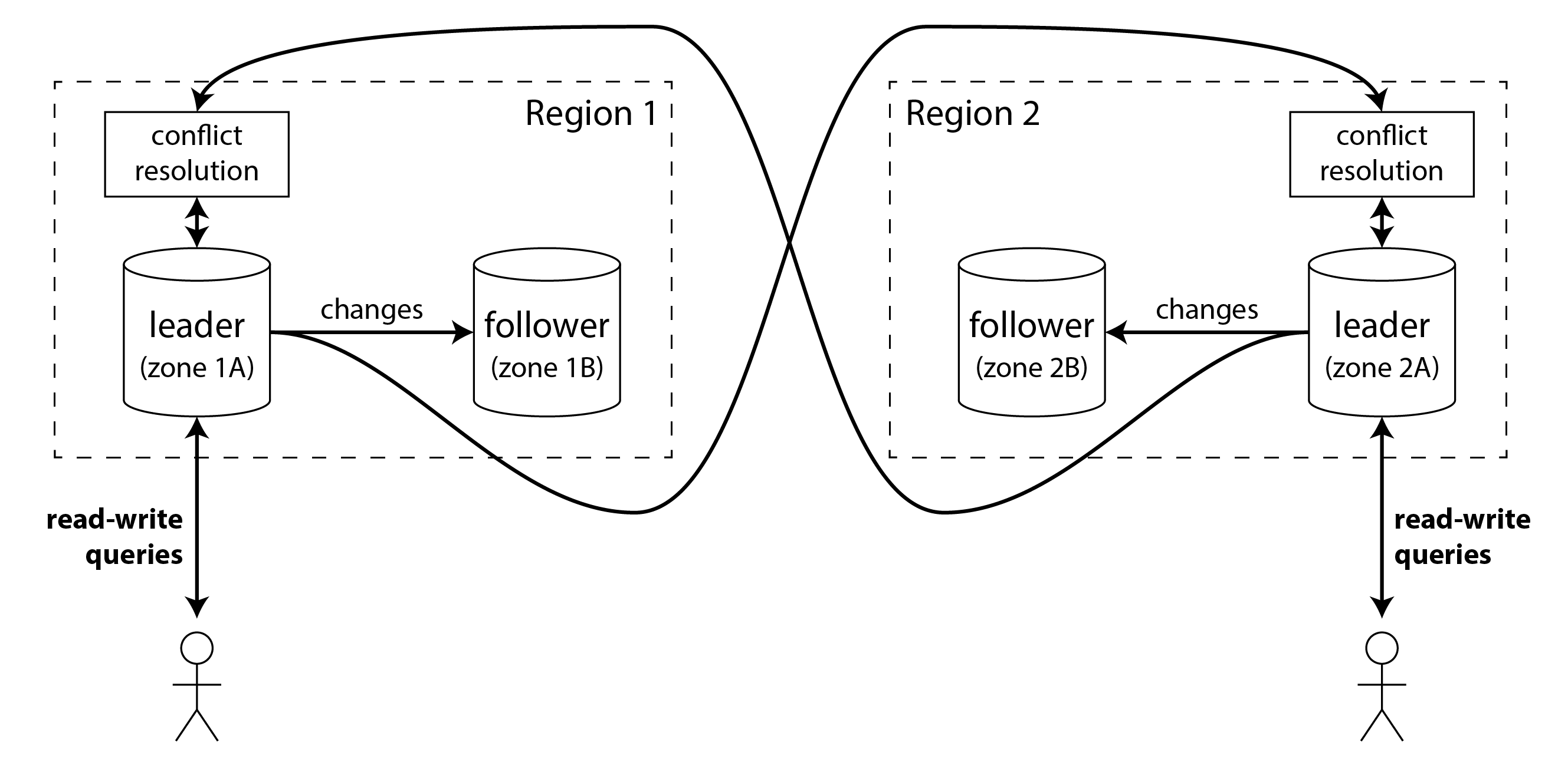
Figure 6-6 Multi-leader replication across multiple regions.

Let’s compare how the single-leader and multi-leader configurations fare in a multi-region deployment:

Performance

In a single-leader configuration, every write must go over the internet to the region with the leader. This can add significant latency to writes and might contravene the purpose of having multiple regions in the first place. In a multi-leader configuration, every write can be processed in the local region and is replicated asynchronously to the other regions. Thus, the inter-region network delay is hidden from users, which means the perceived performance may be better.

Tolerance of regional outages

In a single-leader configuration, if the region with the leader becomes unavailable, failover can promote a follower in another region to be leader. In a multi-leader configuration, each region can continue operating independently of the others, and replication catches up when the offline region comes back online.

Tolerance of network problems

Even with dedicated connections, traffic between regions

can be less reliable than traffic between zones in the same region or within a single zone. A single-leader configuration is very sensitive to problems in this inter-region link, because when a client in one region wants to write to a leader in another region, it has to send its request over that link and wait for the response before it can complete.

A multi-leader configuration with asynchronous replication can tolerate network problems better: during a temporary network interruption, each region’s leader can continue independently processing writes.

Consistency

A single-leader system can provide strong consistency guarantees, such as serializable transactions, which we will discuss in Chapter 8. The biggest downside of multi-leader systems is that the consistency they can achieve is much weaker. For example, you can’t guarantee that a bank account won’t go negative or that a username is unique: it’s always possible for different leaders to process writes that are individually fine (paying out some of the money in an account, registering a particular username), but which violate the constraint when taken together with another write on another leader.

This is simply a fundamental limitation of distributed systems ²⁸. If you need to enforce such constraints, you’re therefore better off with a single-leader system. However, as we will see in “Dealing with Conflicting Writes”, multi-leader systems can still achieve consistency properties that are useful in a wide range of apps that don’t need such constraints.

Multi-leader replication is less common than single-leader replication, but it is still supported by many databases, including MySQL, Oracle, SQL Server, and YugabyteDB. In some cases it is an external add-on feature, for example in Redis Enterprise, EDB Postgres Distributed, and pglogical ²⁹.

As multi-leader replication is a somewhat retrofitted feature in many databases, there are often subtle configuration pitfalls and surprising interactions with other database features. For example, autoincrementing keys, triggers, and integrity constraints can be problematic. For this reason, multi-leader replication is often considered dangerous territory that should be avoided if possible ³⁰.

Multi-leader replication topologies

A replication topology describes the communication paths along which writes are propagated from one node to another. If you have two leaders, like in Figure 6-9, there is only one plausible topology: leader 1 must send all of its writes to leader 2, and vice versa. With more than two leaders, various different topologies are possible. Some examples are illustrated in Figure 6-7.

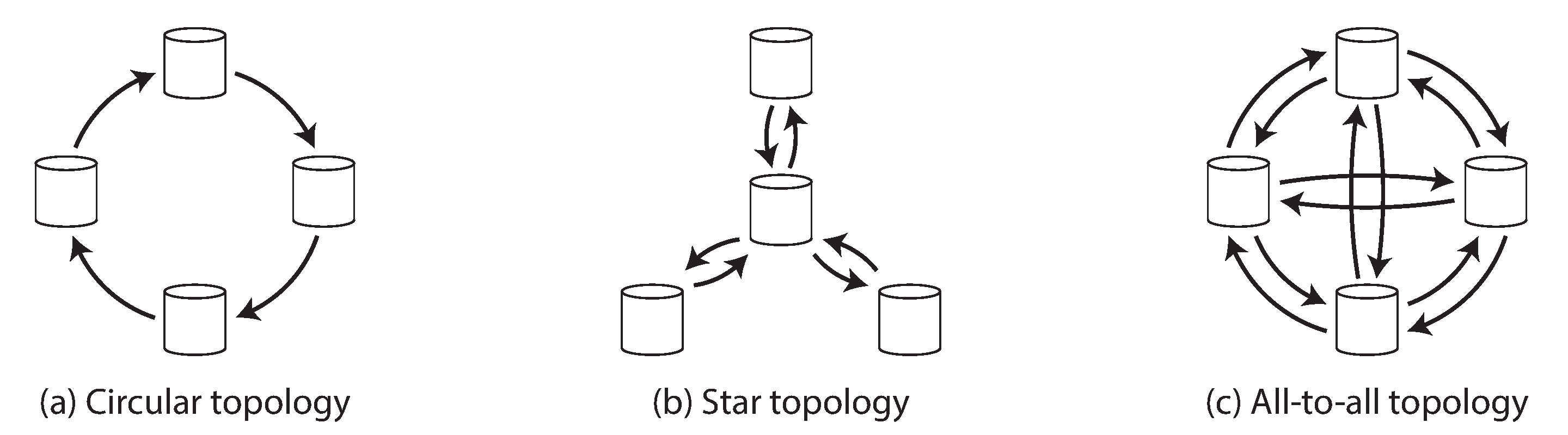
Figure 6-7 Three example topologies in which multi-leader replication can be set up.

The most general topology is all-to-all, shown in Figure 6-7(c), in which every leader sends its writes to every other leader. However, more restricted topologies are also used: for example a circular topology in which each node receives writes from one node and forwards those writes (plus any writes of its own) to one other node. Another popular topology has the shape of a star: one designated root node forwards writes to all of the other nodes. The star topology can be generalized to a tree.

Note

Don’t confuse a star-shaped network topology with a star schema (see “Stars and Snowflakes: Schemas for Analytics”), which describes the structure of a data model.

In circular and star topologies, a write may need to pass through several nodes before it reaches all replicas. Therefore, nodes need to forward data changes they receive from other nodes. To prevent infinite replication loops, each node is given a unique identifier, and in the replication log, each write is tagged with the identifiers of all the nodes it has passed through ³¹. When a node receives a data change that is tagged with its own identifier, that data change is ignored, because the node knows that it has already been processed.

Problems with different topologies

A problem with circular and star topologies is that if just one node fails, it can interrupt the flow of replication messages between other nodes, leaving them unable to communicate until the node is fixed. The topology could be reconfigured to work around the failed node, but in most deployments such reconfiguration would have to be done manually. The fault tolerance of a more densely connected topology (such as all-to-all) is better because it allows messages to travel along different paths, avoiding a single point of failure.

On the other hand, all-to-all topologies can have issues too. In particular, some network links may be faster than others (e.g., due to network congestion), with the result that some replication messages may “overtake” others, as illustrated in Figure 6-8.

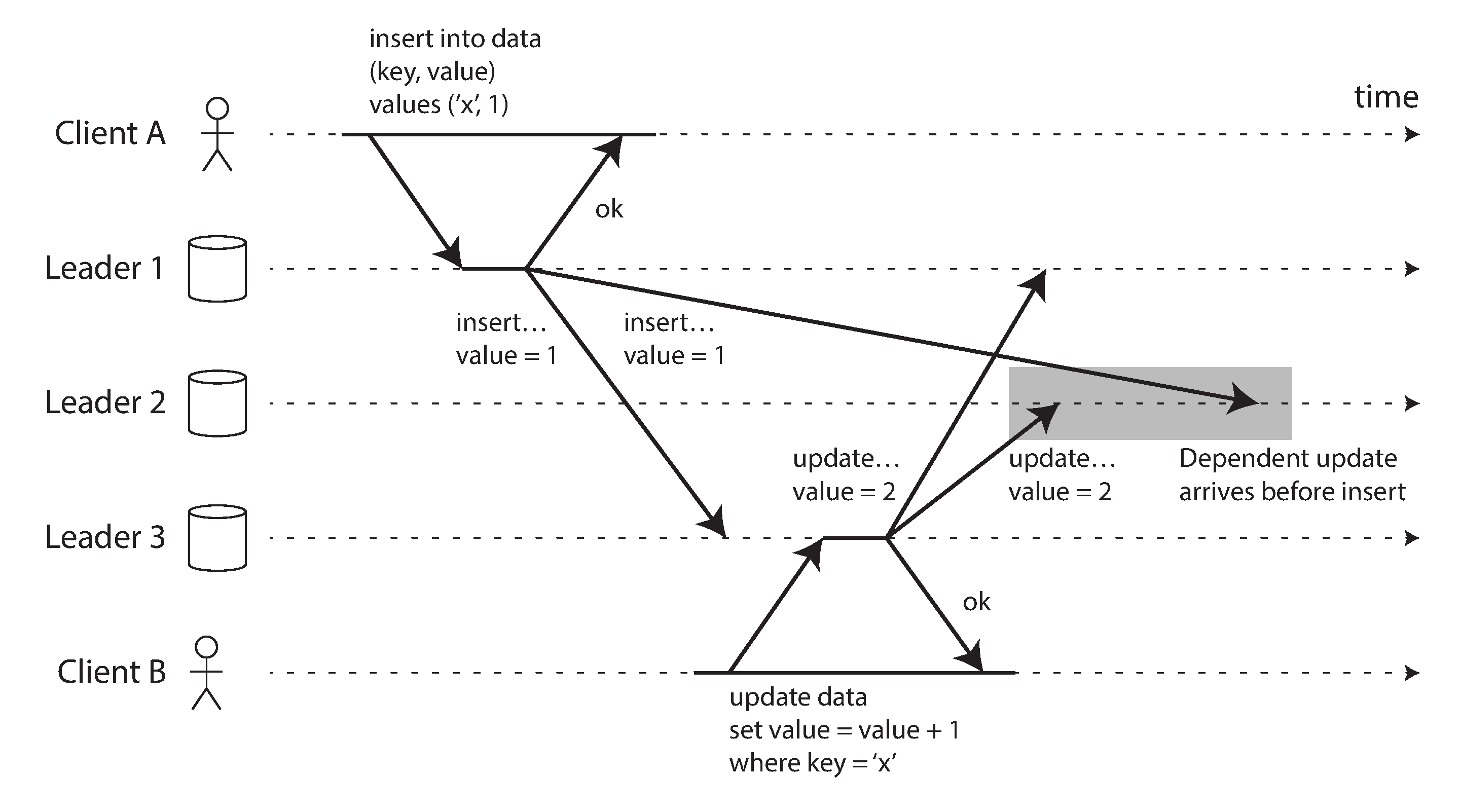
Figure 6-8 With multi-leader replication, writes may arrive in the wrong order at some replicas.

In Figure 6-8, client A inserts a row into a table on leader 1, and client B updates that row on leader 3. However, leader 2 may receive the writes in a different order: it may first receive the update (which, from its point of view, is an update to a row that does not exist in the database) and only later receive the corresponding insert (which should have preceded the update).

This is a problem of causality, similar to the one we saw in “Consistent Prefix Reads”: the update depends on the prior insert, so we need to make sure that all nodes process the insert first, and then the update. Simply attaching a timestamp to every write is not sufficient, because clocks cannot be trusted to be sufficiently in sync to correctly order these events at leader 2 (see Chapter 9).

To order these events correctly, a technique called version vectors can be used, which we will discuss later in this chapter (see “Detecting Concurrent Writes”). However, many multi-leader replication systems don’t use good techniques for ordering updates, leaving them vulnerable to issues like the one in Figure 6-8. If you are using multi-leader replication, it is worth being aware of these issues, carefully reading the documentation, and thoroughly testing your database to ensure that it really does provide the guarantees you believe it to have.

Sync Engines and Local-First Software

Another situation in which multi-leader replication is appropriate is if you have an application that needs to continue to work while it is disconnected from the internet.

For example, consider the calendar apps on your mobile phone, your laptop, and other devices. You need to be able to see your meetings (make read requests) and enter new meetings (make write requests) at any time, regardless of whether your device currently has an internet connection. If you make any changes while you are offline, they need to be synced with a server and your other devices when the device is next online.

In this case, every device has a local database replica that acts as a leader (it accepts write requests), and there is an asynchronous multi-leader replication process (sync) between the replicas of your calendar on all of your devices. The replication lag may be hours or even days, depending on when you have internet access available.

From an architectural point of view, this setup is very similar to multi-leader replication between regions, taken to the extreme: each device is a “region,” and the network connection between them is extremely unreliable.

Real-time collaboration, offline-first, and local-first apps

Moreover, many modern web apps offer real-time collaboration features, such as Google Docs and Sheets for text documents and spreadsheets, Figma for graphics, and Linear for project management. What makes these apps so responsive is that user input is immediately reflected in the user interface, without waiting for a network round-trip to the server, and edits by one user are shown to their collaborators with low latency ³² ³³ ³⁴

This again results in a multi-leader architecture: each web browser tab that has opened the shared file is a replica, and any updates that you make to the file are asynchronously replicated to the devices of the other users who have opened the same file. Even if the app does not allow you to continue editing a file while offline, the fact that multiple users can make edits without waiting for a response from the server already makes it multi-leader.

Both offline editing and real-time collaboration require a similar replication infrastructure: the application needs to capture any changes that the user makes to a file, and either send them to collaborators immediately (if online), or store them locally for sending later (if offline). Additionally, the application needs to receive changes from collaborators, merge them into the user’s local copy of the file, and update the user interface to reflect the latest version. If multiple users have changed the file concurrently, conflict resolution logic may be needed to merge those changes.

A software library that supports this process is called a sync engine. Although the idea has existed for a long time, the term has recently gained attention ³⁵ ³⁶ ³⁷. An application that allows a user to continue editing a file while offline (which may be implemented using a sync engine) is called offline-first ³⁸. The term local-first software refers to collaborative apps that are not only offline-first, but are also designed to continue working even if the developer who made the software shuts down all of their online services ³⁹. This can be achieved by using a sync engine with an open standard sync protocol for which multiple service providers are available ⁴⁰. For example, Git is a local-first collaboration system (albeit one that doesn’t support real-time collaboration) since you can sync via GitHub, GitLab, or any other repository hosting service.

Pros and cons of sync engines

The dominant way of building web apps today is to keep very little persistent state on the client, and to rely on making requests to a server whenever a new piece of data needs to be displayed or some data needs to be updated. In contrast, when using a sync engine, you have persistent state on the client, and communication with the server is moved into a background process. The sync engine approach has a number of advantages:

Having the data locally means the user interface can be much faster to respond than if it had to wait for a service call to fetch some data. Some apps aim to respond to user input in the next frame of the graphics system, which means rendering within 16 ms on a display with a 60 Hz refresh rate.
Allowing users to continue working while offline is valuable, especially on mobile devices with intermittent connectivity. With a sync engine, an app doesn’t need a separate offline mode: being offline is the same as having very large network delay.
A sync engine simplifies the programming model for frontend apps, compared to performing explicit service calls in application code. Every service call requires error handling, as discussed in “The problems with remote procedure calls (RPCs)”: for example, if a request to update data on a server fails, the user interface needs to somehow reflect that error. A sync engine allows the app to perform reads and writes on local data, which almost never fails, leading to a more declarative programming style ⁴¹.
In order to display edits from other users in real-time, you need to receive notifications of those edits and efficiently update the user interface accordingly. A sync engine combined with a reactive programming model is a good way of implementing this ⁴².

Sync engines work best when all the data that the user may need is downloaded in advance and stored persistently on the client. This means that the data is available for offline access when needed, but it also means that sync engines are not suitable if the user has access to a very large amount of data. For example, downloading all the files that the user themselves created is probably fine (one user generally doesn’t generate that much data), but downloading the entire catalog of an e-commerce website probably doesn’t make sense.

The sync engine was pioneered by Lotus Notes in the 1980s ⁴³ (without using that term), and sync for specific apps such as calendars has also existed for a long time. Today there are a number of general-purpose sync engines, some of which use a proprietary backend service (e.g., Google Firestore, Realm, or Ditto), and some have an open source backend, making them suitable for creating local-first software (e.g., PouchDB/CouchDB, Automerge, or Yjs).

Multiplayer video games have a similar need to respond immediately to the user’s local actions, and reconcile them with other players’ actions received asynchronously over the network. In game development jargon the equivalent of a sync engine is called netcode. The techniques used in netcode are quite specific to the requirements of games ⁴⁴, and don’t directly carry over to other types of software, so we won’t consider them further in this book.

Dealing with Conflicting Writes

The biggest problem with multi-leader replication—both in a geo-distributed server-side database and a local-first sync engine on end user devices—is that concurrent writes on different leaders can lead to conflicts that need to be resolved.

For example, consider a wiki page that is simultaneously being edited by two users, as shown in Figure 6-9. User 1 changes the title of the page from A to B, and user 2 independently changes the title from A to C. Each user’s change is successfully applied to their local leader. However, when the changes are asynchronously replicated, a conflict is detected. This problem does not occur in a single-leader database.

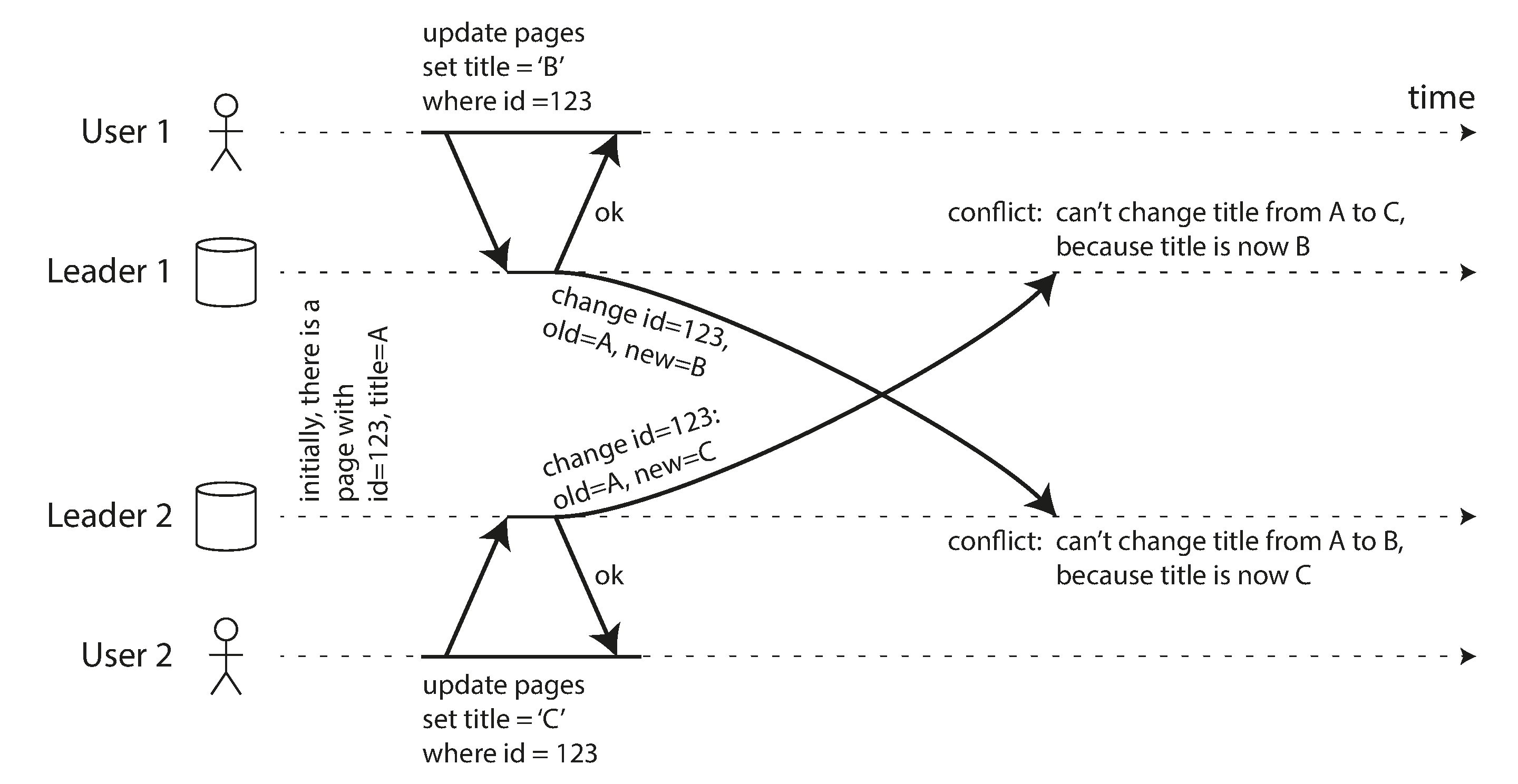
Figure 6-9 A write conflict caused by two leaders concurrently updating the same record.

Note

We say that the two writes in Figure 6-9 are concurrent because neither was “aware” of the other at the time the write was originally made. It doesn’t matter whether the writes literally happened at the same time; indeed, if the writes were made while offline, they might have actually happened some time apart. What matters is whether one write occurred in a state where the other write has already taken effect.

In “Detecting Concurrent Writes” we will tackle the question of how a database can determine whether two writes are concurrent. For now we will assume that we can detect conflicts, and we want to figure out the best way of resolving them.

Conflict avoidance

One strategy for conflicts is to avoid them occurring in the first place. For example, if the application can ensure that all writes for a particular record go through the same leader, then conflicts cannot occur, even if the database as a whole is multi-leader. This approach is not possible in the case of a sync engine client being updated offline, but it is sometimes possible in geo-replicated server systems ³⁰.

For example, in an application where a user can only edit their own data, you can ensure that requests from a particular user are always routed to the same region and use the leader in that region for reading and writing. Different users may have different “home” regions (perhaps picked based on geographic proximity to the user), but from any one user’s point of view the configuration is essentially single-leader.

However, sometimes you might want to change the designated leader for a record—perhaps because one region is unavailable and you need to reroute traffic to another region, or perhaps because a user has moved to a different location and is now closer to a different region. There is now a risk that the user performs a write while the change of designated leader is in progress, leading to a conflict that would have to be resolved using one of the methods below. Thus, conflict avoidance breaks down if you allow the leader to be changed.

Another example of conflict avoidance: imagine you want to insert new records and generate unique IDs for them based on an auto-incrementing counter. If you have two leaders, you could set them up so that one leader only generates odd numbers and the other only generates even numbers. That way you can be sure that the two leaders won’t concurrently assign the same ID to different records. We will discuss other ID assignment schemes in “ID Generators and Logical Clocks”.

Last write wins (discarding concurrent writes)

If conflicts can’t be avoided, the simplest way of resolving them is to attach a timestamp to each write, and to always use the value with the greatest timestamp. For example, in Figure 6-9, let’s say that the timestamp of user 1’s write is greater than the timestamp of user 2’s write. In that case, both leaders will determine that the new title of the page should be B, and they discard the write that sets it to C. If the writes coincidentally have the same timestamp, the winner can be chosen by comparing the values (e.g., in the case of strings, taking the one that’s earlier in the alphabet).

This approach is called last write wins (LWW) because the write with the greatest timestamp can be considered the “last” one. The term is misleading though, because when two writes are concurrent like in Figure 6-9, which one is older and which is later is undefined, and so the timestamp order of concurrent writes is essentially random.

Therefore the real meaning of LWW is: when the same record is concurrently written on different leaders, one of those writes is randomly chosen to be the winner, and the other writes are silently discarded, even though they were successfully processed at their respective leaders. This achieves the goal that eventually all replicas end up in a consistent state, but at the cost of data loss.

If you can avoid conflicts—for example, by only inserting records with a unique key such as a UUID, and never updating them—then LWW is no problem. But if you update existing records, or if different leaders may insert records with the same key, then you have to decide whether lost updates are a problem for your application. If lost updates are not acceptable, you need to use one of the conflict resolution approaches described below.

Another problem with LWW is that if a real-time clock (e.g. a Unix timestamp) is used as timestamp for the writes, the system becomes very sensitive to clock synchronization. If one node has a clock that is ahead of the others, and you try to overwrite a value written by that node, your write may be ignored as it may have a lower timestamp, even though it clearly occurred later. This problem can be solved by using a logical clock, which we will discuss in “ID Generators and Logical Clocks”.

Manual conflict resolution

If randomly discarding some of your writes is not desirable, the next option is to resolve the conflict manually. You may be familiar with manual conflict resolution from Git and other version control systems: if commits on two different branches edit the same lines of the same file, and you try to merge those branches, you will get a merge conflict that needs to be resolved before the merge is complete.

In a database, it would be impractical for a conflict to stop the entire replication process until a human has resolved it. Instead, databases typically store all the concurrently written values for a given record—for example, both B and C in Figure 6-9. These values are sometimes called siblings. The next time you query that record, the database returns all those values, rather than just the latest one. You can then resolve those values in whatever way you want, either automatically in application code (for example, you could concatenate B and C into “B/C”), or by asking the user. You then write back a new value to the database to resolve the conflict.

This approach to conflict resolution is used in some systems, such as CouchDB. However, it also suffers from a number of problems:

The API of the database changes: for example, where previously the title of the wiki page was just a string, it now becomes a set of strings that usually contains one element, but may sometimes contain multiple elements if there is a conflict. This can make the data awkward to work with in application code.
Asking the user to manually merge the siblings is a lot of work, both for the app developer (who needs to build the user interface for conflict resolution) and for the user (who may be confused about what they are being asked to do, and why). In many cases, it’s better to merge automatically than to bother the user.
Merging siblings automatically can lead to surprising behavior if it is not done carefully. For example, the shopping cart on Amazon used to allow concurrent updates, which were then merged by keeping all the shopping cart items that appeared in any of the siblings (i.e., taking the set union of the carts). This meant that if the customer had removed an item from their cart in one sibling, but another sibling still contained that old item, the removed item would unexpectedly reappear in the customer’s cart ⁴⁵. Figure 6-10 shows an example where Device 1 removes Book from the shopping cart and concurrently Device 2 removes DVD, but after merging the conflict both items reappear.
If multiple nodes observe the conflict and concurrently resolve it, the conflict resolution process can itself introduce a new conflict. Those resolutions could even be inconsistent: for example, one node may merge B and C into “B/C” and another may merge them into “C/B” if you are not careful to order them consistently. When the conflict between “B/C” and “C/B” is merged, it may result in “B/C/C/B” or something similarly surprising.

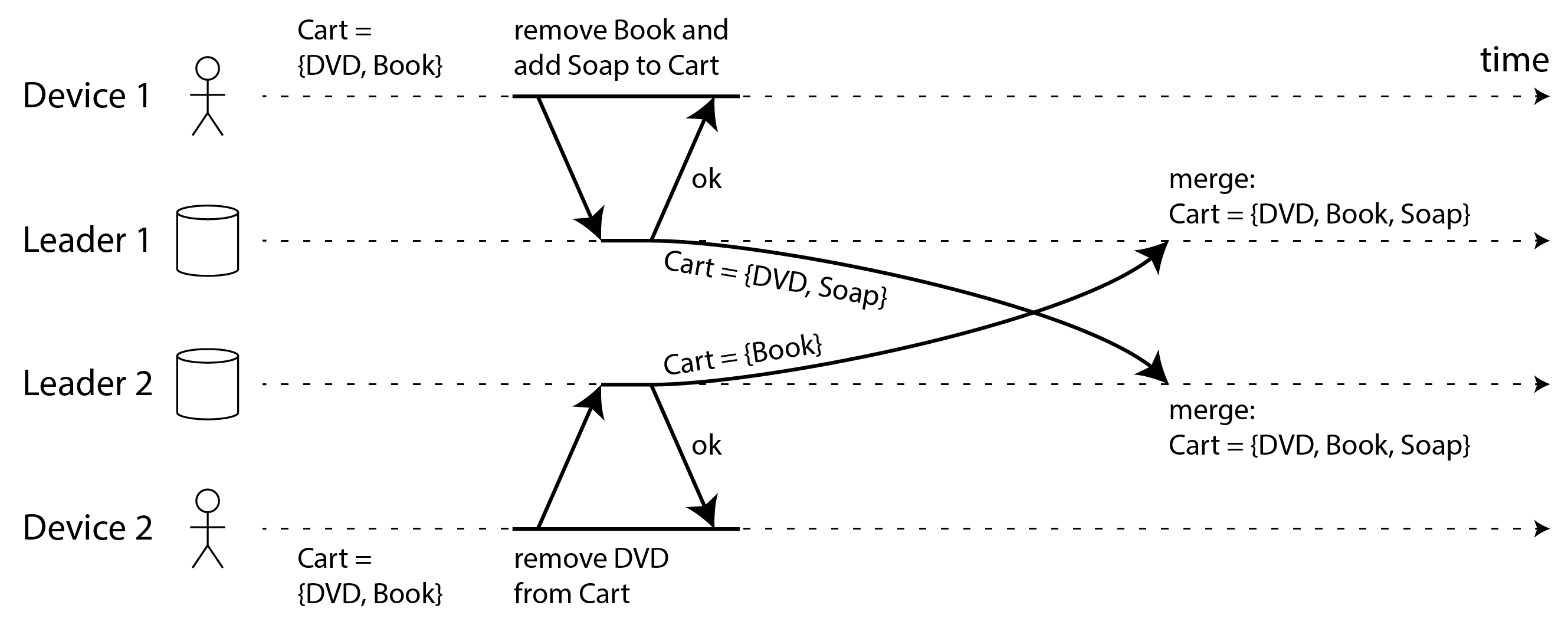
Figure 6-10 Example of Amazon's shopping cart anomaly: if conflicts on a shopping cart are merged by taking the union, deleted items may reappear.

Automatic conflict resolution

For many applications, the best way of handling conflicts is to use an algorithm that automatically merges concurrent writes into a consistent state. Automatic conflict resolution ensures that all replicas converge to the same state—i.e., all replicas that have processed the same set of writes have the same state, regardless of the order in which the writes arrived.

LWW is a simple example of a conflict resolution algorithm. More sophisticated merge algorithms have been developed for different types of data, with the goal of preserving the intended effect of all updates as much as possible, and hence avoiding data loss:

If the data is text (e.g., the title or body of a wiki page), we can detect which characters have been inserted or deleted from one version to the next. The merged result then preserves all the insertions and deletions made in any of the siblings. If users concurrently insert text at the same position, it can be ordered deterministically so that all nodes get the same merged outcome.
If the data is a collection of items (ordered like a to-do list, or unordered like a shopping cart), we can merge it similarly to text by tracking insertions and deletions. To avoid the shopping cart issue in Figure 6-10, the algorithms track the fact that Book and DVD were deleted, so the merged result is Cart = {Soap}.
If the data is an integer representing a counter that can be incremented or decremented (e.g., the number of likes on a social media post), the merge algorithm can tell how many increments and decrements happened on each sibling, and add them together correctly so that the result does not double-count and does not drop updates.
If the data is a key-value mapping, we can merge updates to the same key by applying one of the other conflict resolution algorithms to the values under that key. Updates to different keys can be handled independently from each other.

There are limits to what is possible with conflict resolution. For example, if you want to enforce that a list contains no more than five items, and multiple users concurrently add items to the list so that there are more than five in total, your only option is to drop some of the items. Nevertheless, automatic conflict resolution is sufficient to build many useful apps. And if you start from the requirement of wanting to build a collaborative offline-first or local-first app, then conflict resolution is inevitable, and automating it is often the best approach.

CRDTs and Operational Transformation

Two families of algorithms are commonly used to implement automatic conflict resolution: Conflict-free replicated datatypes (CRDTs) ⁴⁶ and Operational Transformation (OT) ⁴⁷. They have different design philosophies and performance characteristics, but both are able to perform automatic merges for all the aforementioned types of data.

Figure 6-11 shows an example of how OT and a CRDT merge concurrent updates to a text. Assume you have two replicas that both start off with the text “ice”. One replica prepends the letter “n” to make “nice”, while concurrently the other replica appends an exclamation mark to make “ice!”.

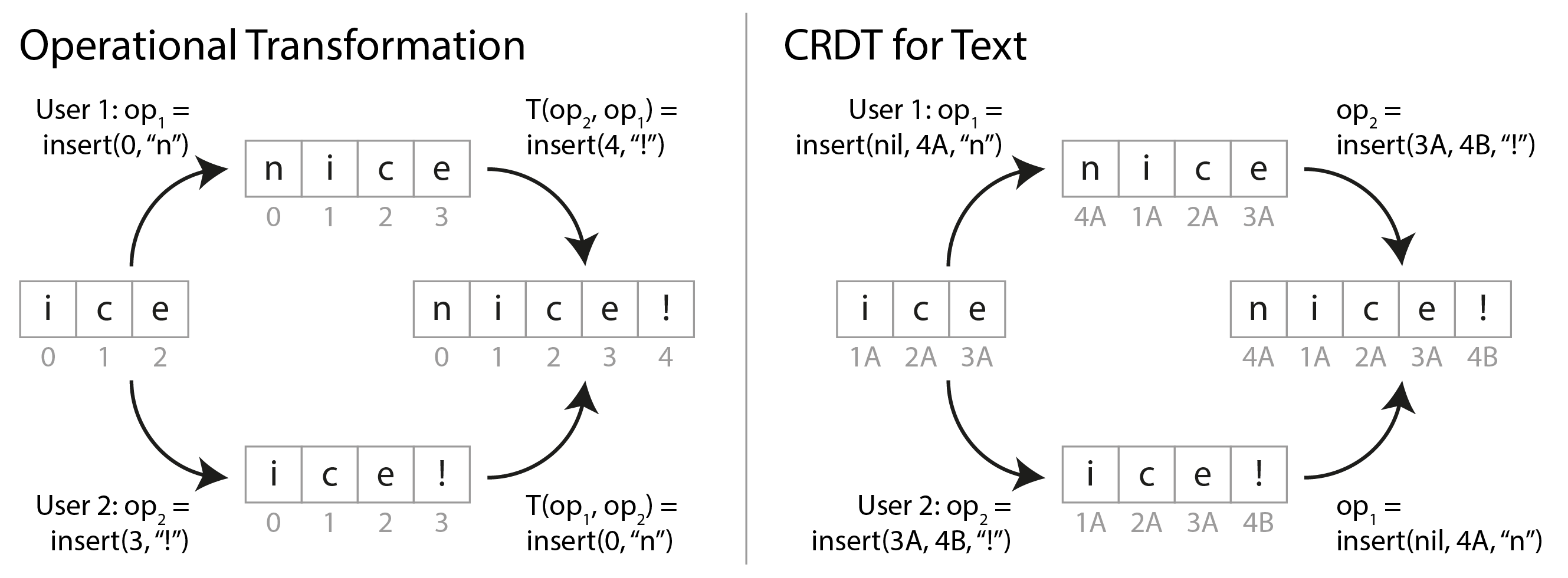
Figure 6-11 How two concurrent insertions into a string are merged by OT and a CRDT respectively.

The merged result “nice!” is achieved differently by both types of algorithms:

OT: We record the index at which characters are inserted or deleted: “n” is inserted at index 0, and “!” at index 3. Next, the replicas exchange their operations. The insertion of “n” at 0 can be applied as-is, but if the insertion of “!” at 3 were applied to the state “nice” we would get “nic!e”, which is incorrect. We therefore need to transform the index of each operation to account for concurrent operations that have already been applied; in this case, the insertion of “!” is transformed to index 4 to account for the insertion of “n” at an earlier index.
CRDT: Most CRDTs give each character a unique, immutable ID and use those to determine the positions of insertions/deletions, instead of indexes. For example, in Figure 6-11 we assign the ID 1A to “i”, the ID 2A to “c”, etc. When inserting the exclamation mark, we generate an operation containing the ID of the new character (4B) and the ID of the existing character after which we want to insert (3A). To insert at the beginning of the string we give “nil” as the preceding character ID. Concurrent insertions at the same position are ordered by the IDs of the characters. This ensures that replicas converge without performing any transformation.

There are many algorithms based on variations of these ideas. Lists/arrays can be supported similarly, using list elements instead of characters, and other datatypes such as key-value maps can be added quite easily. There are some performance and functionality trade-offs between OT and CRDTs, but it’s possible to combine the advantages of CRDTs and OT in one algorithm ⁴⁸.

OT is most often used for real-time collaborative editing of text, e.g. in Google Docs ³², whereas CRDTs can be found in distributed databases such as Redis Enterprise, Riak, and Azure Cosmos DB ⁴⁹. Sync engines for JSON data can be implemented both with CRDTs (e.g., Automerge or Yjs) and with OT (e.g., ShareDB).

What is a conflict?

Some kinds of conflict are obvious. In the example in Figure 6-9, two writes concurrently modified the same field in the same record, setting it to two different values. There is little doubt that this is a conflict.

Other kinds of conflict can be more subtle to detect. For example, consider a meeting room booking system: it tracks which room is booked by which group of people at which time. This application needs to ensure that each room is only booked by one group of people at any one time (i.e., there must not be any overlapping bookings for the same room). In this case, a conflict may arise if two different bookings are created for the same room at the same time. Even if the application checks availability before allowing a user to make a booking, there can be a conflict if the two bookings are made on two different leaders.

There isn’t a quick ready-made answer, but in the following chapters we will trace a path toward a good understanding of this problem. We will see some more examples of conflicts in Chapter 8, and in “Ordering events to capture causality” we will discuss scalable approaches for detecting and resolving conflicts in a replicated system.

Leaderless Replication

The replication approaches we have discussed so far in this chapter—single-leader and multi-leader replication—are based on the idea that a client sends a write request to one node (the leader), and the database system takes care of copying that write to the other replicas. A leader determines the order in which writes should be processed, and followers apply the leader’s writes in the same order.

Some data storage systems take a different approach, abandoning the concept of a leader and allowing any replica to directly accept writes from clients. Some of the earliest replicated data systems were leaderless ¹ ⁵⁰, but the idea was mostly forgotten during the era of dominance of relational databases. It once again became a fashionable architecture for databases after Amazon used it for its in-house Dynamo system in 2007 ⁴⁵. Riak, Cassandra, and ScyllaDB are open source datastores with leaderless replication models inspired by Dynamo, so this kind of database is also known as Dynamo-style.

Note

The original Dynamo system was only described in a paper ⁴⁵, but never released outside of Amazon. The similarly-named DynamoDB is a more recent cloud database from AWS, but it has a completely different architecture: it uses single-leader replication based on the Multi-Paxos consensus algorithm ⁵.

In some leaderless implementations, the client directly sends its writes to several replicas, while in others, a coordinator node does this on behalf of the client. However, unlike a leader database, that coordinator does not enforce a particular ordering of writes. As we shall see, this difference in design has profound consequences for the way the database is used.

Writing to the Database When a Node Is Down

Imagine you have a database with three replicas, and one of the replicas is currently unavailable—perhaps it is being rebooted to install a system update. In a single-leader configuration, if you want to continue processing writes, you may need to perform a failover (see “Handling Node Outages”).

On the other hand, in a leaderless configuration, failover does not exist. Figure 6-12 shows what happens: the client (user 1234) sends the write to all three replicas in parallel, and the two available replicas accept the write but the unavailable replica misses it. Let’s say that it’s sufficient for two out of three replicas to acknowledge the write: after user 1234 has received two ok responses, we consider the write to be successful. The client simply ignores the fact that one of the replicas missed the write.

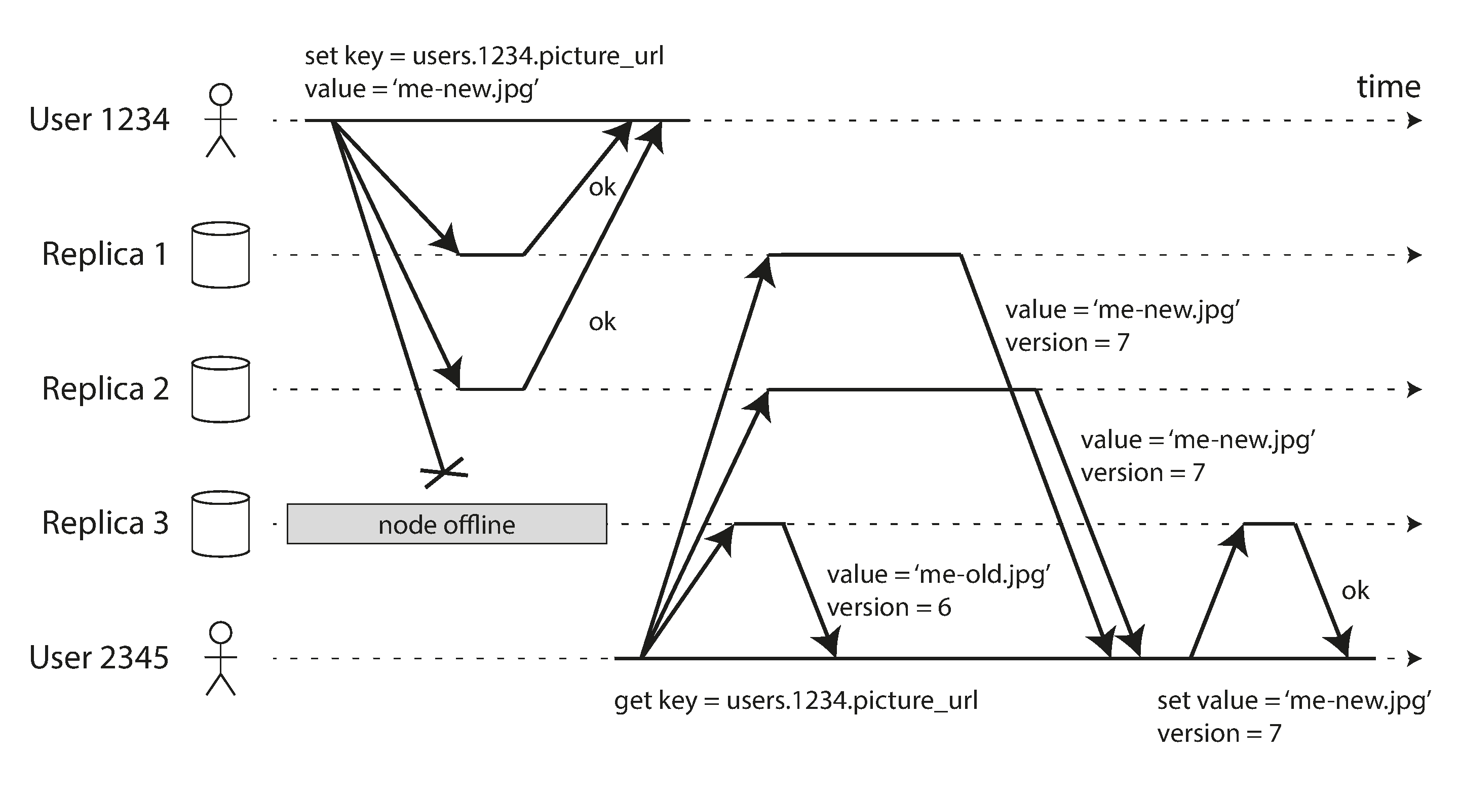
Figure 6-12 A quorum write, quorum read, and read repair after a node outage.

Now imagine that the unavailable node comes back online, and clients start reading from it. Any writes that happened while the node was down are missing from that node. Thus, if you read from that node, you may get stale (outdated) values as responses.

To solve that problem, when a client reads from the database, it doesn’t just send its request to one replica: read requests are also sent to several nodes in parallel. The client may get different responses from different nodes; for example, the up-to-date value from one node and a stale value from another.

In order to tell which responses are up-to-date and which are outdated, every value that is written needs to be tagged with a version number or timestamp, similarly to what we saw in “Last write wins (discarding concurrent writes)”. When a client receives multiple values in response to a read, it uses the one with the greatest timestamp (even if that value was only returned by one replica, and several other replicas returned older values). See “Detecting Concurrent Writes” for more details.

Catching up on missed writes

The replication system should ensure that eventually all the data is copied to every replica. After an unavailable node comes back online, how does it catch up on the writes that it missed? Several mechanisms are used in Dynamo-style datastores:

Read repair: When a client makes a read from several nodes in parallel, it can detect any stale responses. For example, in Figure 6-12, user 2345 gets a version 6 value from replica 3 and a version 7 value from replicas 1 and 2. The client sees that replica 3 has a stale value and writes the newer value back to that replica. This approach works well for values that are frequently read.
Hinted handoff: If one replica is unavailable, another replica may store writes on its behalf in the form of hints. When the replica that was supposed to receive those writes comes back, the replica storing the hints sends them to the recovered replica, and then deletes the hints. This handoff process helps bring replicas up-to-date even for values that are never read, and therefore not handled by read repair.
Anti-entropy: In addition, there is a background process that periodically looks for differences in the data between replicas and copies any missing data from one replica to another. Unlike the replication log in leader-based replication, this anti-entropy process does not copy writes in any particular order, and there may be a significant delay before data is copied.

Quorums for reading and writing

In the example of Figure 6-12, we considered the write to be successful even though it was only processed on two out of three replicas. What if only one out of three replicas accepted the write? How far can we push this?

If we know that every successful write is guaranteed to be present on at least two out of three replicas, that means at most one replica can be stale. Thus, if we read from at least two replicas, we can be sure that at least one of the two is up to date. If the third replica is down or slow to respond, reads can nevertheless continue returning an up-to-date value.

More generally, if there are n replicas, every write must be confirmed by w nodes to be considered successful, and we must query at least r nodes for each read. (In our example, n = 3, w = 2, r = 2.) As long as w + r > n, we expect to get an up-to-date value when reading, because at least one of the r nodes we’re reading from must be up to date. Reads and writes that obey these r and w values are called quorum reads and writes ⁵⁰. You can think of r and w as the minimum number of votes required for the read or write to be valid.

In Dynamo-style databases, the parameters n, w, and r are typically configurable. A common choice is to make n an odd number (typically 3 or 5) and to set w = r = (n + 1) / 2 (rounded up). However, you can vary the numbers as you see fit. For example, a workload with few writes and many reads may benefit from setting w = n and r = 1. This makes reads faster, but has the disadvantage that just one failed node causes all database writes to fail.

Note

There may be more than n nodes in the cluster, but any given value is stored only on n nodes. This allows the dataset to be sharded, supporting datasets that are larger than you can fit on one node. We will return to sharding in Chapter 7.

The quorum condition, w + r > n, allows the system to tolerate unavailable nodes as follows:

If w < n, we can still process writes if a node is unavailable.
If r < n, we can still process reads if a node is unavailable.
With n = 3, w = 2, r = 2 we can tolerate one unavailable node, like in Figure 6-12.
With n = 5, w = 3, r = 3 we can tolerate two unavailable nodes. This case is illustrated in Figure 6-13.

Normally, reads and writes are always sent to all n replicas in parallel. The parameters w and r determine how many nodes we wait for—i.e., how many of the n nodes need to report success before we consider the read or write to be successful.

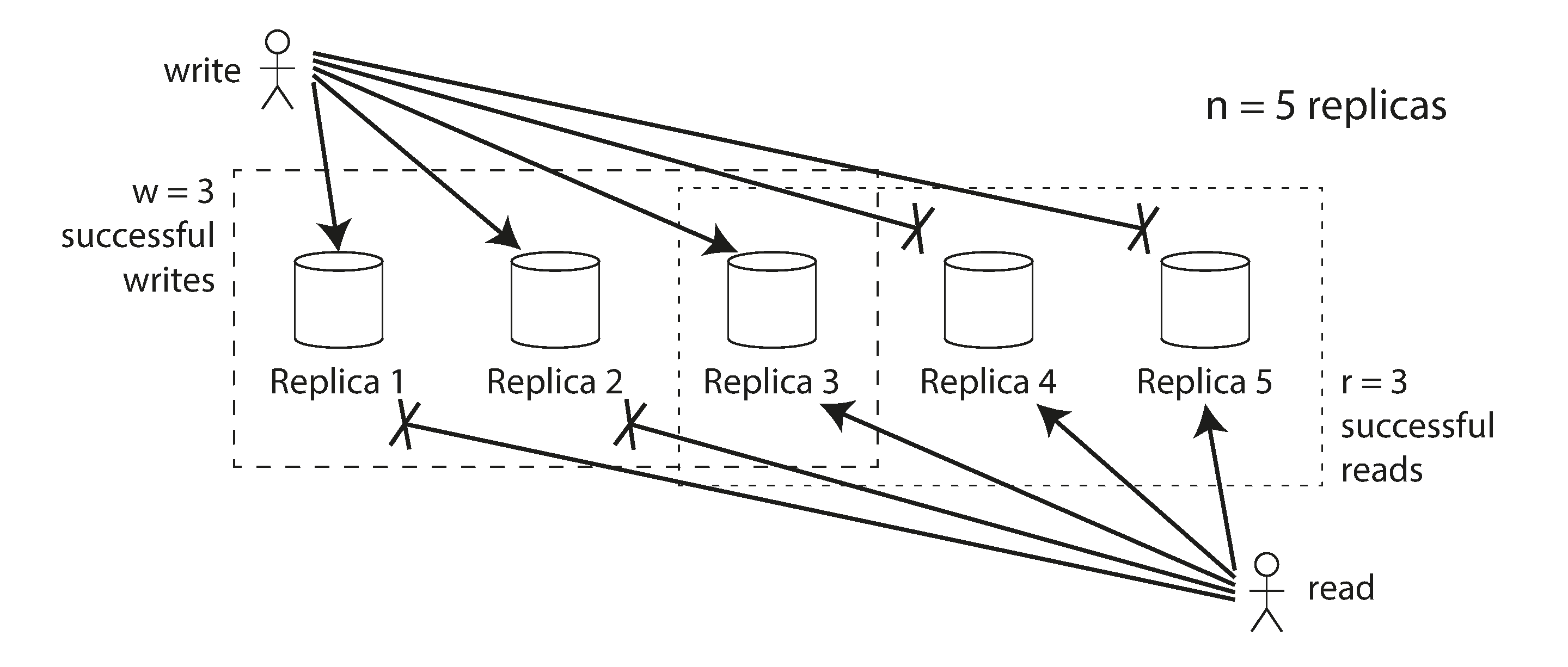
Figure 6-13 If w + r > n, at least one of the r replicas you read from must have seen the most recent successful write.

If fewer than the required w or r nodes are available, writes or reads return an error. A node could be unavailable for many reasons: because the node is down (crashed, powered down), due to an error executing the operation (can’t write because the disk is full), due to a network interruption between the client and the node, or for any number of other reasons. We only care whether the node returned a successful response and don’t need to distinguish between different kinds of fault.

Limitations of Quorum Consistency

If you have n replicas, and you choose w and r such that w + r > n, you can generally expect every read to return the most recent value written for a key. This is the case because the set of nodes to which you’ve written and the set of nodes from which you’ve read must overlap. That is, among the nodes you read there must be at least one node with the latest value (illustrated in Figure 6-13).

Often, r and w are chosen to be a majority (more than n/2) of nodes, because that ensures w + r > n while still tolerating up to n/2 (rounded down) node failures. But quorums are not necessarily majorities—it only matters that the sets of nodes used by the read and write operations overlap in at least one node. Other quorum assignments are possible, which allows some flexibility in the design of distributed algorithms ⁵¹.

You may also set w and r to smaller numbers, so that w + r ≤ n (i.e., the quorum condition is not satisfied). In this case, reads and writes will still be sent to n nodes, but a smaller number of successful responses is required for the operation to succeed.

With a smaller w and r you are more likely to read stale values, because it’s more likely that your read didn’t include the node with the latest value. On the upside, this configuration allows lower latency and higher availability: if there is a network interruption and many replicas become unreachable, there’s a higher chance that you can continue processing reads and writes. Only after the number of reachable replicas falls below w or r does the database become unavailable for writing or reading, respectively.

However, even with w + r > n, there are edge cases in which the consistency properties can be confusing. Some scenarios include:

If a node carrying a new value fails, and its data is restored from a replica carrying an old value, the number of replicas storing the new value may fall below w, breaking the quorum condition.
While a rebalancing is in progress, where some data is moved from one node to another (see Chapter 7), nodes may have inconsistent views of which nodes should be holding the n replicas for a particular value. This can result in the read and write quorums no longer overlapping.
If a read is concurrent with a write operation, the read may or may not see the concurrently written value. In particular, it’s possible for one read to see the new value, and a subsequent read to see the old value, as we shall see in “Linearizability and quorums”.
If a write succeeded on some replicas but failed on others (for example because the disks on some nodes are full), and overall succeeded on fewer than w replicas, it is not rolled back on the replicas where it succeeded. This means that if a write was reported as failed, subsequent reads may or may not return the value from that write ⁵².
If the database uses timestamps from a real-time clock to determine which write is newer (as Cassandra and ScyllaDB do, for example), writes might be silently dropped if another node with a faster clock has written to the same key—an issue we previously saw in “Last write wins (discarding concurrent writes)”. We will discuss this in more detail in “Relying on Synchronized Clocks”.
If two writes occur concurrently, one of them might be processed first on one replica, and the other might be processed first on another replica. This leads to a conflict, similarly to what we saw for multi-leader replication (see “Dealing with Conflicting Writes”). We will return to this topic in “Detecting Concurrent Writes”.

Thus, although quorums appear to guarantee that a read returns the latest written value, in practice it is not so simple. Dynamo-style databases are generally optimized for use cases that can tolerate eventual consistency. The parameters w and r allow you to adjust the probability of stale values being read ⁵³, but it’s wise to not take them as absolute guarantees.

Monitoring staleness

From an operational perspective, it’s important to monitor whether your databases are returning up-to-date results. Even if your application can tolerate stale reads, you need to be aware of the health of your replication. If it falls behind significantly, it should alert you so that you can investigate the cause (for example, a problem in the network or an overloaded node).

For leader-based replication, the database typically exposes metrics for the replication lag, which you can feed into a monitoring system. This is possible because writes are applied to the leader and to followers in the same order, and each node has a position in the replication log (the number of writes it has applied locally). By subtracting a follower’s current position from the leader’s current position, you can measure the amount of replication lag.

However, in systems with leaderless replication, there is no fixed order in which writes are applied, which makes monitoring more difficult. The number of hints that a replica stores for handoff can be one measure of system health, but it’s difficult to interpret usefully ⁵⁴. Eventual consistency is a deliberately vague guarantee, but for operability it’s important to be able to quantify “eventual.”

Single-Leader vs. Leaderless Replication Performance

A replication system based on a single leader can provide strong consistency guarantees that are difficult or impossible to achieve in a leaderless system. However, as we have seen in “Problems with Replication Lag”, reads in a leader-based replicated system can also return stale values if you make them on an asynchronously updated follower.

Reading from the leader ensures up-to-date responses, but it suffers from performance problems:

Read throughput is limited by the leader’s capacity to handle requests (in contrast with read scaling, which distributes reads across asynchronously updated replicas that may return stale values).
If the leader fails, you have to wait for the fault to be detected, and for the failover to complete before you can continue handling requests. Even if the failover process is very quick, users will notice it because of the temporarily increased response times; if failover takes a long time, the system is unavailable for its duration.
The system is very sensitive to performance problems on the leader: if the leader is slow to respond, e.g. due to overload or some resource contention, the increased response times immediately affect users as well.

A big advantage of a leaderless architecture is that it is more resilient against such issues. Because there is no failover, and requests go to multiple replicas in parallel anyway, one replica becoming slow or unavailable has very little impact on response times: the client simply uses the responses from the other replicas that are faster to respond. Using the fastest responses is called request hedging, and it can significantly reduce tail latency ⁵⁵).

At its core, the resilience of a leaderless system comes from the fact that it doesn’t distinguish between the normal case and the failure case. This is especially helpful when handling so-called gray failures, in which a node isn’t completely down, but running in a degraded state where it is unusually slow to handle requests ⁵⁶, or when a node is simply overloaded (for example, if a node has been offline for a while, recovery via hinted handoff can cause a lot of additional load). A leader-based system has to decide whether the situation is bad enough to warrant a failover (which can itself cause further disruption), whereas in a leaderless system that question doesn’t even arise.

That said, leaderless systems can have performance problems as well:

Even though the system doesn’t need to perform failover, one replica does need to detect when another replica is unavailable so that it can store hints about writes that the unavailable replica missed. When the unavailable replica comes back, the handoff process needs to send it those hints. This puts additional load on the replicas at a time when the system is already under strain ⁵⁴.
The more replicas you have, the bigger the size of your quorums, and the more responses you have to wait for before a request can complete. Even if you wait only for the fastest r or w replicas to respond, and even if you make the requests in parallel, a bigger r or w increases the chance that you hit a slow replica, increasing the overall response time (see “Use of Response Time Metrics”).
A large-scale network interruption that disconnects a client from a large number of replicas can make it impossible to form a quorum. Some leaderless databases offer a configuration option that allows any reachable replica to accept writes, even if it’s not one of the usual replicas for that key (Riak and Dynamo call this a sloppy quorum ⁴⁵; Cassandra and ScyllaDB call it consistency level ANY). There is no guarantee that subsequent reads will see the written value, but depending on the application it may still be better than having the write fail.

Multi-leader replication can offer even greater resilience against network interruptions than leaderless replication, since reads and writes only require communication with one leader, which can be co-located with the client. However, since a write on one leader is propagated asynchronously to the others, reads can be arbitrarily out-of-date. Quorum reads and writes provide a compromise: good fault tolerance while also having a high likelihood of reading up-to-date data.

Multi-region operation

We previously discussed cross-region replication as a use case for multi-leader replication (see “Multi-Leader Replication”). Leaderless replication is also suitable for multi-region operation, since it is designed to tolerate conflicting concurrent writes, network interruptions, and latency spikes.

Cassandra and ScyllaDB implement their multi-region support within the normal leaderless model: the client sends its writes directly to the replicas in all regions, and you can choose from a variety of consistency levels that determine how many responses are required for a request to be successful. For example, you can request a quorum across the replicas in all the regions, a separate quorum in each of the regions, or a quorum only in the client’s local region. A local quorum avoids having to wait for slow requests to other regions, but it is also more likely to return stale results.

Riak keeps all communication between clients and database nodes local to one region, so n describes the number of replicas within one region. Cross-region replication between database clusters happens asynchronously in the background, in a style that is similar to multi-leader replication.

Detecting Concurrent Writes

Like with multi-leader replication, leaderless databases allow concurrent writes to the same key, resulting in conflicts that need to be resolved. Such conflicts may occur as the writes happen, but not always: they could also be detected later during read repair, hinted handoff, or anti-entropy.

The problem is that events may arrive in a different order at different nodes, due to variable network delays and partial failures. For example, Figure 6-14 shows two clients, A and B, simultaneously writing to a key X in a three-node datastore:

Node 1 receives the write from A, but never receives the write from B due to a transient outage.
Node 2 first receives the write from A, then the write from B.
Node 3 first receives the write from B, then the write from A.

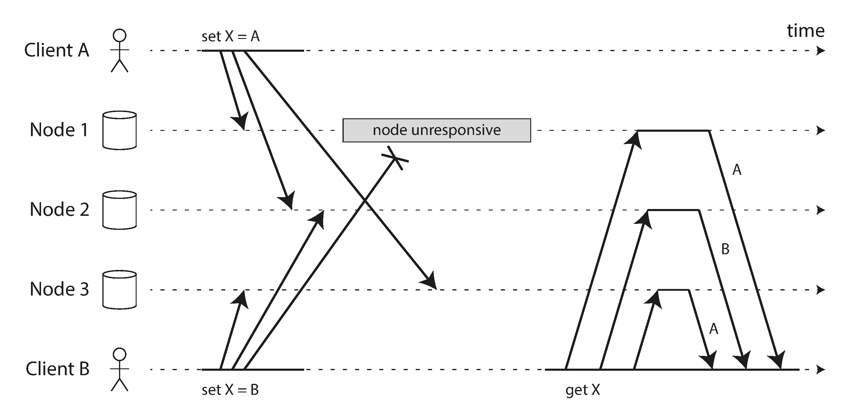
Figure 6-14 Concurrent writes in a Dynamo-style datastore: there is no well-defined ordering.

If each node simply overwrote the value for a key whenever it received a write request from a client, the nodes would become permanently inconsistent, as shown by the final get request in Figure 6-14: node 2 thinks that the final value of X is B, whereas the other nodes think that the value is A.

In order to become eventually consistent, the replicas should converge toward the same value. For this, we can use any of the conflict resolution mechanisms we previously discussed in “Dealing with Conflicting Writes”, such as last-write-wins (used by Cassandra and ScyllaDB), manual resolution, or CRDTs (described in “CRDTs and Operational Transformation”, and used by Riak).

Last-write-wins is easy to implement: each write is tagged with a timestamp, and a value with a higher timestamp always overwrites a value with a lower timestamp. However, a timestamp doesn’t tell you whether two values are actually conflicting (i.e., they were written concurrently) or not (they were written one after another). If you want to resolve conflicts explicitly, the system needs to take more care to detect concurrent writes.

The “happens-before” relation and concurrency

How do we decide whether two operations are concurrent or not? To develop an intuition, let’s look at some examples:

In Figure 6-8, the two writes are not concurrent: A’s insert happens before B’s increment, because the value incremented by B is the value inserted by A. In other words, B’s operation builds upon A’s operation, so B’s operation must have happened later. We also say that B is causally dependent on A.
On the other hand, the two writes in Figure 6-14 are concurrent: when each client starts the operation, it does not know that another client is also performing an operation on the same key. Thus, there is no causal dependency between the operations.

An operation A happens before another operation B if B knows about A, or depends on A, or builds upon A in some way. Whether one operation happens before another operation is the key to defining what concurrency means. In fact, we can simply say that two operations are concurrent if neither happens before the other (i.e., neither knows about the other) ⁵⁷.

Thus, whenever you have two operations A and B, there are three possibilities: either A happened before B, or B happened before A, or A and B are concurrent. What we need is an algorithm to tell us whether two operations are concurrent or not. If one operation happened before another, the later operation should overwrite the earlier operation, but if the operations are concurrent, we have a conflict that needs to be resolved.

![TIP] Concurrency, Time, and Relativity

It may seem that two operations should be called concurrent if they occur “at the same time”—but in fact, it is not important whether they literally overlap in time. Because of problems with clocks in distributed systems, it is actually quite difficult to tell whether two things happened at exactly the same time—an issue we will discuss in more detail in Chapter 9.

For defining concurrency, exact time doesn’t matter: we simply call two operations concurrent if they are both unaware of each other, regardless of the physical time at which they occurred. People sometimes make a connection between this principle and the special theory of relativity in physics ⁵⁷, which introduced the idea that information cannot travel faster than the speed of light. Consequently, two events that occur some distance apart cannot possibly affect each other if the time between the events is shorter than the time it takes light to travel the distance between them.

In computer systems, two operations might be concurrent even though the speed of light would in principle have allowed one operation to affect the other. For example, if the network was slow or interrupted at the time, two operations can occur some time apart and still be concurrent, because the network problems prevented one operation from being able to know about the other.

Capturing the happens-before relationship

Let’s look at an algorithm that determines whether two operations are concurrent, or whether one happened before another. To keep things simple, let’s start with a database that has only one replica. Once we have worked out how to do this on a single replica, we can generalize the approach to a leaderless database with multiple replicas.

Figure 6-15 shows two clients concurrently adding items to the same shopping cart. (If that example strikes you as too inane, imagine instead two air traffic controllers concurrently adding aircraft to the sector they are tracking.) Initially, the cart is empty. Between them, the clients make five writes to the database:

Client 1 adds milk to the cart. This is the first write to that key, so the server successfully stores it and assigns it version 1. The server also echoes the value back to the client, along with the version number.
Client 2 adds eggs to the cart, not knowing that client 1 concurrently added milk (client 2 thought that its eggs were the only item in the cart). The server assigns version 2 to this write, and stores eggs and milk as two separate values (siblings). It then returns both values to the client, along with the version number of 2.
Client 1, oblivious to client 2’s write, wants to add flour to the cart, so it thinks the current cart contents should be [milk, flour]. It sends this value to the server, along with the version number 1 that the server gave client 1 previously. The server can tell from the version number that the write of [milk, flour] supersedes the prior value of [milk] but that it is concurrent with [eggs]. Thus, the server assigns version 3 to [milk, flour], overwrites the version 1 value [milk], but keeps the version 2 value [eggs] and returns both remaining values to the client.
Meanwhile, client 2 wants to add ham to the cart, unaware that client 1 just added flour. Client 2 received the two values [milk] and [eggs] from the server in the last response, so the client now merges those values and adds ham to form a new value, [eggs, milk, ham]. It sends that value to the server, along with the previous version number 2. The server detects that version 2 overwrites [eggs] but is concurrent with [milk, flour], so the two remaining values are [milk, flour] with version 3, and [eggs, milk, ham] with version 4.
Finally, client 1 wants to add bacon. It previously received [milk, flour] and [eggs] from the server at version 3, so it merges those, adds bacon, and sends the final value [milk, flour, eggs, bacon] to the server, along with the version number 3. This overwrites [milk, flour] (note that [eggs] was already overwritten in the last step) but is concurrent with [eggs, milk, ham], so the server keeps those two concurrent values.

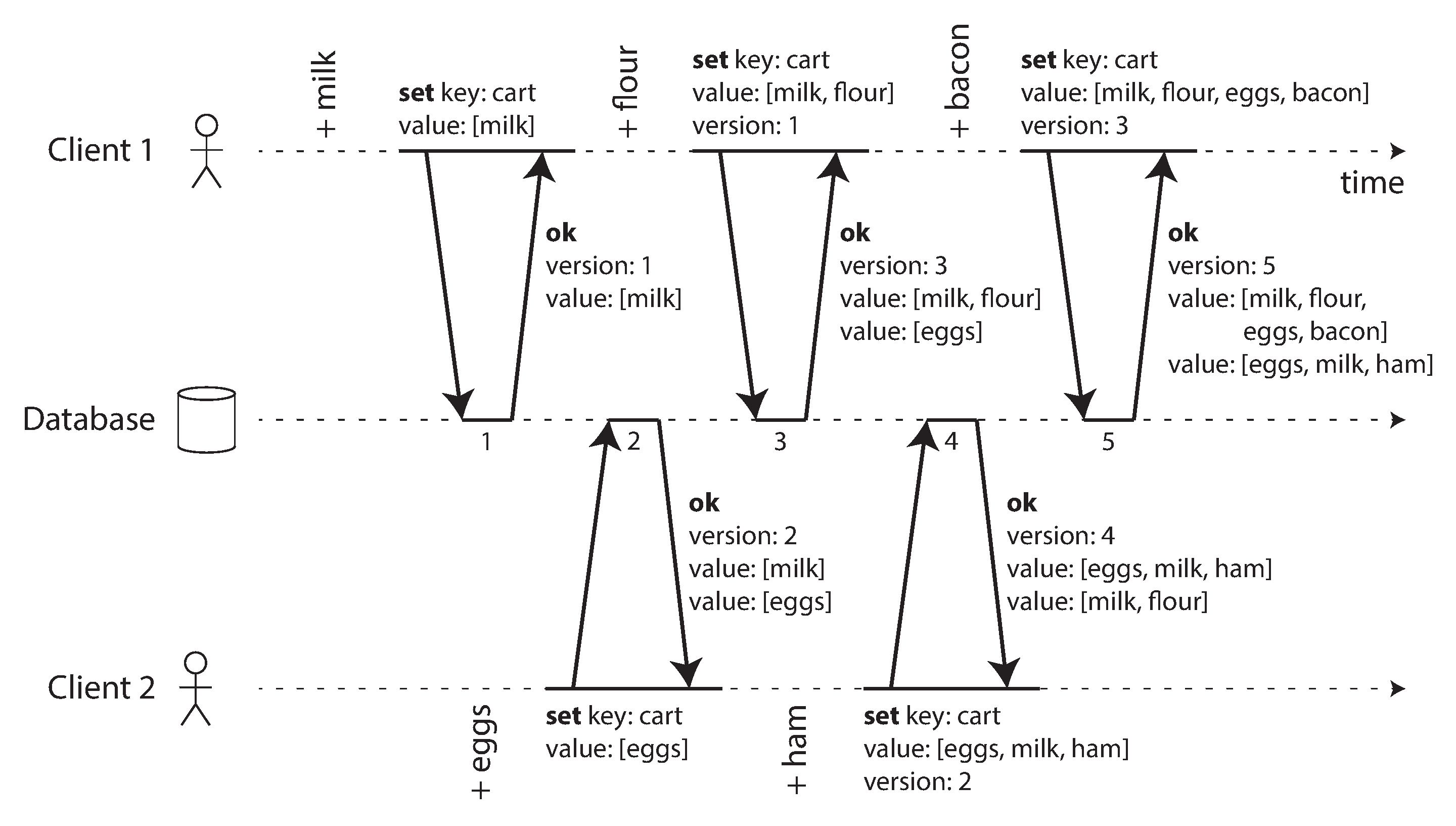
Figure 6-15 Capturing causal dependencies between two clients concurrently editing a shopping cart.

The dataflow between the operations in Figure 6-15 is illustrated graphically in Figure 6-16. The arrows indicate which operation happened before which other operation, in the sense that the later operation knew about or depended on the earlier one. In this example, the clients are never fully up to date with the data on the server, since there is always another operation going on concurrently. But old versions of the value do get overwritten eventually, and no writes are lost.

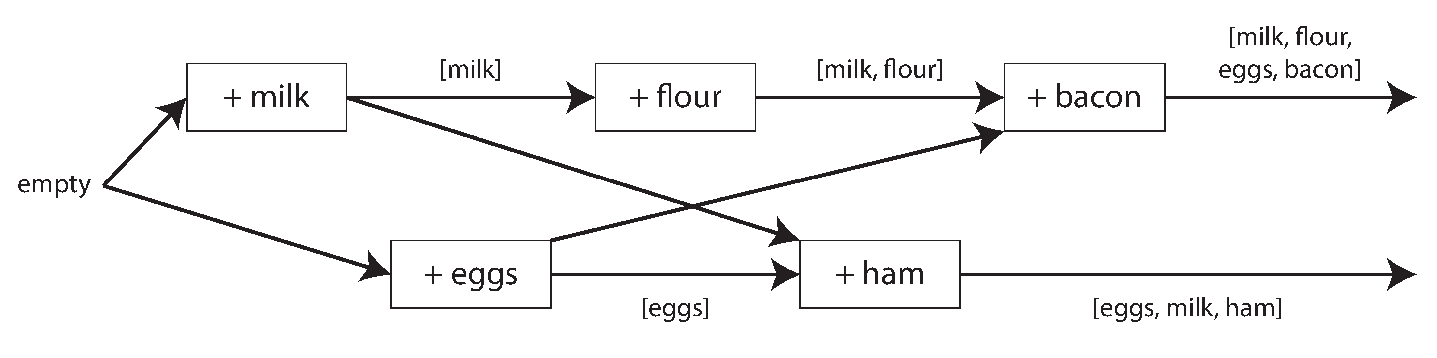
Figure 6-16 Graph of causal dependencies in Figure 6-15.

Note that the server can determine whether two operations are concurrent by looking at the version numbers—it does not need to interpret the value itself (so the value could be any data structure). The algorithm works as follows:

The server maintains a version number for every key, increments the version number every time that key is written, and stores the new version number along with the value written.
When a client reads a key, the server returns all siblings, i.e., all values that have not been overwritten, as well as the latest version number. A client must read a key before writing.
When a client writes a key, it must include the version number from the prior read, and it must merge together all values that it received in the prior read, e.g. using a CRDT or by asking the user. The response from a write request is like a read, returning all siblings, which allows us to chain several writes like in the shopping cart example.
When the server receives a write with a particular version number, it can overwrite all values with that version number or below (since it knows that they have been merged into the new value), but it must keep all values with a higher version number (because those values are concurrent with the incoming write).

When a write includes the version number from a prior read, that tells us which previous state the write is based on. If you make a write without including a version number, it is concurrent with all other writes, so it will not overwrite anything—it will just be returned as one of the values on subsequent reads.

Version vectors

The example in Figure 6-15 used only a single replica. How does the algorithm change when there are multiple replicas, but no leader?

Figure 6-15 uses a single version number to capture dependencies between operations, but that is not sufficient when there are multiple replicas accepting writes concurrently. Instead, we need to use a version number per replica as well as per key. Each replica increments its own version number when processing a write, and also keeps track of the version numbers it has seen from each of the other replicas. This information indicates which values to overwrite and which values to keep as siblings.

The collection of version numbers from all the replicas is called a version vector ⁵⁸. A few variants of this idea are in use, but the most interesting is probably the dotted version vector ⁵⁹ ⁶⁰, which is used in Riak 2.0 ⁶¹ ⁶². We won’t go into the details, but the way it works is quite similar to what we saw in our cart example.

Like the version numbers in Figure 6-15, version vectors are sent from the database replicas to clients when values are read, and need to be sent back to the database when a value is subsequently written. (Riak encodes the version vector as a string that it calls causal context.) The version vector allows the database to distinguish between overwrites and concurrent writes.

The version vector also ensures that it is safe to read from one replica and subsequently write back to another replica. Doing so may result in siblings being created, but no data is lost as long as siblings are merged correctly.

VERSION VECTORS AND VECTOR CLOCKS

A version vector is sometimes also called a vector clock, even though they are not quite the same. The difference is subtle—please see the references for details ⁶⁰ ⁶³ ⁶⁴. In brief, when comparing the state of replicas, version vectors are the right data structure to use.

Summary

In this chapter we looked at the issue of replication. Replication can serve several purposes:

High availability: Keeping the system running, even when one machine (or several machines, a zone, or even an entire region) goes down
Disconnected operation: Allowing an application to continue working when there is a network interruption
Latency: Placing data geographically close to users, so that users can interact with it faster
Scalability: Being able to handle a higher volume of reads than a single machine could handle, by performing reads on replicas

Despite being a simple goal—keeping a copy of the same data on several machines—replication turns out to be a remarkably tricky problem. It requires carefully thinking about concurrency and about all the things that can go wrong, and dealing with the consequences of those faults. At a minimum, we need to deal with unavailable nodes and network interruptions (and that’s not even considering the more insidious kinds of fault, such as silent data corruption due to software bugs or hardware errors).

We discussed three main approaches to replication:

Single-leader replication: Clients send all writes to a single node (the leader), which sends a stream of data change events to the other replicas (followers). Reads can be performed on any replica, but reads from followers might be stale.
Multi-leader replication: Clients send each write to one of several leader nodes, any of which can accept writes. The leaders send streams of data change events to each other and to any follower nodes.
Leaderless replication: Clients send each write to several nodes, and read from several nodes in parallel in order to detect and correct nodes with stale data.

Each approach has advantages and disadvantages. Single-leader replication is popular because it is fairly easy to understand and it offers strong consistency. Multi-leader and leaderless replication can be more robust in the presence of faulty nodes, network interruptions, and latency spikes—at the cost of requiring conflict resolution and providing weaker consistency guarantees.

Replication can be synchronous or asynchronous, which has a profound effect on the system behavior when there is a fault. Although asynchronous replication can be fast when the system is running smoothly, it’s important to figure out what happens when replication lag increases and servers fail. If a leader fails and you promote an asynchronously updated follower to be the new leader, recently committed data may be lost.

We looked at some strange effects that can be caused by replication lag, and we discussed a few consistency models which are helpful for deciding how an application should behave under replication lag:

Read-after-write consistency: Users should always see data that they submitted themselves.
Monotonic reads: After users have seen the data at one point in time, they shouldn’t later see the data from some earlier point in time.
Consistent prefix reads: Users should see the data in a state that makes causal sense: for example, seeing a question and its reply in the correct order.

Finally, we discussed how multi-leader and leaderless replication ensure that all replicas eventually converge to a consistent state: by using a version vector or similar algorithm to detect which writes are concurrent, and by using a conflict resolution algorithm such as a CRDT to merge the concurrently written values. Last-write-wins and manual conflict resolution are also possible.

This chapter has assumed that every replica stores a full copy of the whole database, which is unrealistic for large datasets. In the next chapter we will look at sharding, which allows each machine to store only a subset of the data.

References

B. G. Lindsay, P. G. Selinger, C. Galtieri, J. N. Gray, R. A. Lorie, T. G. Price, F. Putzolu, I. L. Traiger, and B. W. Wade. Notes on Distributed Databases. IBM Research, Research Report RJ2571(33471), July 1979. Archived at perma.cc/EPZ3-MHDD ↩︎ ↩︎
Kenny Gryp. MySQL Terminology Updates. dev.mysql.com, July 2020. Archived at perma.cc/S62G-6RJ2 ↩︎
Oracle Corporation. Oracle (Active) Data Guard 19c: Real-Time Data Protection and Availability. White Paper, oracle.com, March 2019. Archived at perma.cc/P5ST-RPKE ↩︎
Microsoft. What is an Always On availability group? learn.microsoft.com, September 2024. Archived at perma.cc/ABH6-3MXF ↩︎
Mostafa Elhemali, Niall Gallagher, Nicholas Gordon, Joseph Idziorek, Richard Krog, Colin Lazier, Erben Mo, Akhilesh Mritunjai, Somu Perianayagam, Tim Rath, Swami Sivasubramanian, James Christopher Sorenson III, Sroaj Sosothikul, Doug Terry, and Akshat Vig. Amazon DynamoDB: A Scalable, Predictably Performant, and Fully Managed NoSQL Database Service. At USENIX Annual Technical Conference (ATC), July 2022. ↩︎ ↩︎
Rebecca Taft, Irfan Sharif, Andrei Matei, Nathan VanBenschoten, Jordan Lewis, Tobias Grieger, Kai Niemi, Andy Woods, Anne Birzin, Raphael Poss, Paul Bardea, Amruta Ranade, Ben Darnell, Bram Gruneir, Justin Jaffray, Lucy Zhang, and Peter Mattis. CockroachDB: The Resilient Geo-Distributed SQL Database. At ACM SIGMOD International Conference on Management of Data (SIGMOD), pages 1493–1509, June 2020. doi:10.1145/3318464.3386134 ↩︎
Dongxu Huang, Qi Liu, Qiu Cui, Zhuhe Fang, Xiaoyu Ma, Fei Xu, Li Shen, Liu Tang, Yuxing Zhou, Menglong Huang, Wan Wei, Cong Liu, Jian Zhang, Jianjun Li, Xuelian Wu, Lingyu Song, Ruoxi Sun, Shuaipeng Yu, Lei Zhao, Nicholas Cameron, Liquan Pei, and Xin Tang. TiDB: a Raft-based HTAP database. Proceedings of the VLDB Endowment, volume 13, issue 12, pages 3072–3084. doi:10.14778/3415478.3415535 ↩︎
Mallory Knodel and Niels ten Oever. Terminology, Power, and Inclusive Language in Internet-Drafts and RFCs. IETF Internet-Draft, August 2023. Archived at perma.cc/5ZY9-725E ↩︎
Buck Hodges. Postmortem: VSTS 4 September 2018. devblogs.microsoft.com, September 2018. Archived at perma.cc/ZF5R-DYZS ↩︎
Gunnar Morling. Leader Election With S3 Conditional Writes. www.morling.dev, August 2024. Archived at perma.cc/7V2N-J78Y ↩︎
Vignesh Chandramohan, Rohan Desai, and Chris Riccomini. SlateDB Manifest Design. github.com, May 2024. Archived at perma.cc/8EUY-P32Z ↩︎
Stas Kelvich. Why does Neon use Paxos instead of Raft, and what’s the difference? neon.tech, August 2022. Archived at perma.cc/SEZ4-2GXU ↩︎
Dimitri Fontaine. An introduction to the pg_auto_failover project. tapoueh.org, November 2021. Archived at perma.cc/3WH5-6BAF ↩︎
Jesse Newland. GitHub availability this week. github.blog, September 2012. Archived at perma.cc/3YRF-FTFJ ↩︎
Mark Imbriaco. Downtime last Saturday. github.blog, December 2012. Archived at perma.cc/M7X5-E8SQ ↩︎
John Hugg. ‘All In’ with Determinism for Performance and Testing in Distributed Systems. At Strange Loop, September 2015. ↩︎
Hironobu Suzuki. The Internals of PostgreSQL. interdb.jp, 2017. ↩︎
Amit Kapila. WAL Internals of PostgreSQL. At PostgreSQL Conference (PGCon), May 2012. Archived at perma.cc/6225-3SUX ↩︎
Amit Kapila. Evolution of Logical Replication. amitkapila16.blogspot.com, September 2023. Archived at perma.cc/F9VX-JLER ↩︎
Aru Petchimuthu. Upgrade your Amazon RDS for PostgreSQL or Amazon Aurora PostgreSQL database, Part 2: Using the pglogical extension. aws.amazon.com, August 2021. Archived at perma.cc/RXT8-FS2T ↩︎
Yogeshwer Sharma, Philippe Ajoux, Petchean Ang, David Callies, Abhishek Choudhary, Laurent Demailly, Thomas Fersch, Liat Atsmon Guz, Andrzej Kotulski, Sachin Kulkarni, Sanjeev Kumar, Harry Li, Jun Li, Evgeniy Makeev, Kowshik Prakasam, Robbert van Renesse, Sabyasachi Roy, Pratyush Seth, Yee Jiun Song, Benjamin Wester, Kaushik Veeraraghavan, and Peter Xie. Wormhole: Reliable Pub-Sub to Support Geo-Replicated Internet Services. At 12th USENIX Symposium on Networked Systems Design and Implementation (NSDI), May 2015. ↩︎
Douglas B. Terry. Replicated Data Consistency Explained Through Baseball. Microsoft Research, Technical Report MSR-TR-2011-137, October 2011. Archived at perma.cc/F4KZ-AR38 ↩︎ ↩︎ ↩︎
Douglas B. Terry, Alan J. Demers, Karin Petersen, Mike J. Spreitzer, Marvin M. Theher, and Brent B. Welch. Session Guarantees for Weakly Consistent Replicated Data. At 3rd International Conference on Parallel and Distributed Information Systems (PDIS), September 1994. doi:10.1109/PDIS.1994.331722 ↩︎ ↩︎
Werner Vogels. Eventually Consistent. ACM Queue, volume 6, issue 6, pages 14–19, October 2008. doi:10.1145/1466443.1466448 ↩︎
Simon Willison. Reply to: “My thoughts about Fly.io (so far) and other newish technology I’m getting into”. news.ycombinator.com, May 2022. Archived at perma.cc/ZRV4-WWV8 ↩︎
Nithin Tharakan. Scaling Bitbucket’s Database. atlassian.com, October 2020. Archived at perma.cc/JAB7-9FGX ↩︎
Terry Pratchett. Reaper Man: A Discworld Novel. Victor Gollancz, 1991. ISBN: 978-0-575-04979-6 ↩︎
Peter Bailis, Alan Fekete, Michael J. Franklin, Ali Ghodsi, Joseph M. Hellerstein, and Ion Stoica. Coordination Avoidance in Database Systems. Proceedings of the VLDB Endowment, volume 8, issue 3, pages 185–196, November 2014. doi:10.14778/2735508.2735509 ↩︎
Yaser Raja and Peter Celentano. PostgreSQL bi-directional replication using pglogical. aws.amazon.com, January 2022. Archived at https://perma.cc/BUQ2-5QWN ↩︎
Robert Hodges. If You *Must* Deploy Multi-Master Replication, Read This First. scale-out-blog.blogspot.com, April 2012. Archived at perma.cc/C2JN-F6Y8 ↩︎ ↩︎
Lars Hofhansl. HBASE-7709: Infinite Loop Possible in Master/Master Replication. issues.apache.org, January 2013. Archived at perma.cc/24G2-8NLC ↩︎
John Day-Richter. What’s Different About the New Google Docs: Making Collaboration Fast. drive.googleblog.com, September 2010. Archived at perma.cc/5TL8-TSJ2 ↩︎ ↩︎
Evan Wallace. How Figma’s multiplayer technology works. figma.com, October 2019. Archived at perma.cc/L49H-LY4D ↩︎
Tuomas Artman. Scaling the Linear Sync Engine. linear.app, June 2023. ↩︎
Amr Saafan. Why Sync Engines Might Be the Future of Web Applications. nilebits.com, September 2024. Archived at perma.cc/5N73-5M3V ↩︎
Isaac Hagoel. Are Sync Engines The Future of Web Applications? dev.to, July 2024. Archived at perma.cc/R9HF-BKKL ↩︎
Sujay Jayakar. A Map of Sync. stack.convex.dev, October 2024. Archived at perma.cc/82R3-H42A ↩︎
Alex Feyerke. Designing Offline-First Web Apps. alistapart.com, December 2013. Archived at perma.cc/WH7R-S2DS ↩︎
Martin Kleppmann, Adam Wiggins, Peter van Hardenberg, and Mark McGranaghan. Local-first software: You own your data, in spite of the cloud. At ACM SIGPLAN International Symposium on New Ideas, New Paradigms, and Reflections on Programming and Software (Onward!), October 2019, pages 154–178. doi:10.1145/3359591.3359737 ↩︎
Martin Kleppmann. The past, present, and future of local-first. At Local-First Conference, May 2024. ↩︎
Conrad Hofmeyr. API Calling is to Sync Engines as jQuery is to React. powersync.com, November 2024. Archived at perma.cc/2FP9-7WJJ ↩︎
Peter van Hardenberg and Martin Kleppmann. PushPin: Towards Production-Quality Peer-to-Peer Collaboration. At 7th Workshop on Principles and Practice of Consistency for Distributed Data (PaPoC), April 2020. doi:10.1145/3380787.3393683 ↩︎
Leonard Kawell, Jr., Steven Beckhardt, Timothy Halvorsen, Raymond Ozzie, and Irene Greif. Replicated document management in a group communication system. At ACM Conference on Computer-Supported Cooperative Work (CSCW), September 1988. doi:10.1145/62266.1024798 ↩︎
Ricky Pusch. Explaining how fighting games use delay-based and rollback netcode. words.infil.net and arstechnica.com, October 2019. Archived at perma.cc/DE7W-RDJ8 ↩︎
Giuseppe DeCandia, Deniz Hastorun, Madan Jampani, Gunavardhan Kakulapati, Avinash Lakshman, Alex Pilchin, Swaminathan Sivasubramanian, Peter Vosshall, and Werner Vogels. Dynamo: Amazon’s Highly Available Key-Value Store. At 21st ACM Symposium on Operating Systems Principles (SOSP), October 2007. doi:10.1145/1323293.1294281 ↩︎ ↩︎ ↩︎ ↩︎
Marc Shapiro, Nuno Preguiça, Carlos Baquero, and Marek Zawirski. A Comprehensive Study of Convergent and Commutative Replicated Data Types. INRIA Research Report no. 7506, January 2011. ↩︎
Chengzheng Sun and Clarence Ellis. Operational Transformation in Real-Time Group Editors: Issues, Algorithms, and Achievements. At ACM Conference on Computer Supported Cooperative Work (CSCW), November 1998. doi:10.1145/289444.289469 ↩︎
Joseph Gentle and Martin Kleppmann. Collaborative Text Editing with Eg-walker: Better, Faster, Smaller. At 20th European Conference on Computer Systems (EuroSys), March 2025. doi:10.1145/3689031.3696076 ↩︎
Dharma Shukla. Azure Cosmos DB: Pushing the frontier of globally distributed databases. azure.microsoft.com, September 2018. Archived at perma.cc/UT3B-HH6R ↩︎
David K. Gifford. Weighted Voting for Replicated Data. At 7th ACM Symposium on Operating Systems Principles (SOSP), December 1979. doi:10.1145/800215.806583 ↩︎ ↩︎
Heidi Howard, Dahlia Malkhi, and Alexander Spiegelman. Flexible Paxos: Quorum Intersection Revisited. At 20th International Conference on Principles of Distributed Systems (OPODIS), December 2016. doi:10.4230/LIPIcs.OPODIS.2016.25 ↩︎
Joseph Blomstedt. Bringing Consistency to Riak. At RICON West, October 2012. ↩︎
Peter Bailis, Shivaram Venkataraman, Michael J. Franklin, Joseph M. Hellerstein, and Ion Stoica. Quantifying eventual consistency with PBS. The VLDB Journal, volume 23, pages 279–302, April 2014. doi:10.1007/s00778-013-0330-1 ↩︎
Colin Breck. Shared-Nothing Architectures for Server Replication and Synchronization. blog.colinbreck.com, December 2019. Archived at perma.cc/48P3-J6CJ ↩︎ ↩︎
Jeffrey Dean and Luiz André Barroso. The Tail at Scale. Communications of the ACM, volume 56, issue 2, pages 74–80, February 2013. doi:10.1145/2408776.2408794 ↩︎
Peng Huang, Chuanxiong Guo, Lidong Zhou, Jacob R. Lorch, Yingnong Dang, Murali Chintalapati, and Randolph Yao. Gray Failure: The Achilles’ Heel of Cloud-Scale Systems. At 16th Workshop on Hot Topics in Operating Systems (HotOS), May 2017. doi:10.1145/3102980.3103005 ↩︎
Leslie Lamport. Time, Clocks, and the Ordering of Events in a Distributed System. Communications of the ACM, volume 21, issue 7, pages 558–565, July 1978. doi:10.1145/359545.359563 ↩︎ ↩︎
D. Stott Parker Jr., Gerald J. Popek, Gerard Rudisin, Allen Stoughton, Bruce J. Walker, Evelyn Walton, Johanna M. Chow, David Edwards, Stephen Kiser, and Charles Kline. Detection of Mutual Inconsistency in Distributed Systems. IEEE Transactions on Software Engineering, volume SE-9, issue 3, pages 240–247, May 1983. doi:10.1109/TSE.1983.236733 ↩︎
Nuno Preguiça, Carlos Baquero, Paulo Sérgio Almeida, Victor Fonte, and Ricardo Gonçalves. Dotted Version Vectors: Logical Clocks for Optimistic Replication. arXiv:1011.5808, November 2010. ↩︎
Giridhar Manepalli. Clocks and Causality - Ordering Events in Distributed Systems. exhypothesi.com, November 2022. Archived at perma.cc/8REU-KVLQ ↩︎ ↩︎
Sean Cribbs. A Brief History of Time in Riak. At RICON, October 2014. Archived at perma.cc/7U9P-6JFX ↩︎
Russell Brown. Vector Clocks Revisited Part 2: Dotted Version Vectors. riak.com, November 2015. Archived at perma.cc/96QP-W98R ↩︎
Carlos Baquero. Version Vectors Are Not Vector Clocks. haslab.wordpress.com, July 2011. Archived at perma.cc/7PNU-4AMG ↩︎
Reinhard Schwarz and Friedemann Mattern. Detecting Causal Relationships in Distributed Computations: In Search of the Holy Grail. Distributed Computing, volume 7, issue 3, pages 149–174, March 1994. doi:10.1007/BF02277859 ↩︎

7. Sharding

Clearly, we must break away from the sequential and not limit the computers. We must state definitions and provide for priorities and descriptions of data. We must state relationships, not procedures.

Grace Murray Hopper, Management and the Computer of the Future (1962)

A distributed database typically distributes data across nodes in two ways:

Having a copy of the same data on multiple nodes: this is replication, which we discussed in Chapter 6.
If we don’t want every node to store all the data, we can split up a large amount of data into smaller shards or partitions, and store different shards on different nodes. We’ll discuss sharding in this chapter.

Normally, shards are defined in such a way that each piece of data (each record, row, or document) belongs to exactly one shard. There are various ways of achieving this, which we discuss in depth in this chapter. In effect, each shard is a small database of its own, although some database systems support operations that touch multiple shards at the same time.

Sharding is usually combined with replication so that copies of each shard are stored on multiple nodes. This means that, even though each record belongs to exactly one shard, it may still be stored on several different nodes for fault tolerance.

A node may store more than one shard. If a single-leader replication model is used, the combination of sharding and replication can look like Figure 7-1, for example. Each shard’s leader is assigned to one node, and its followers are assigned to other nodes. Each node may be the leader for some shards and a follower for other shards, but each shard still only has one leader.

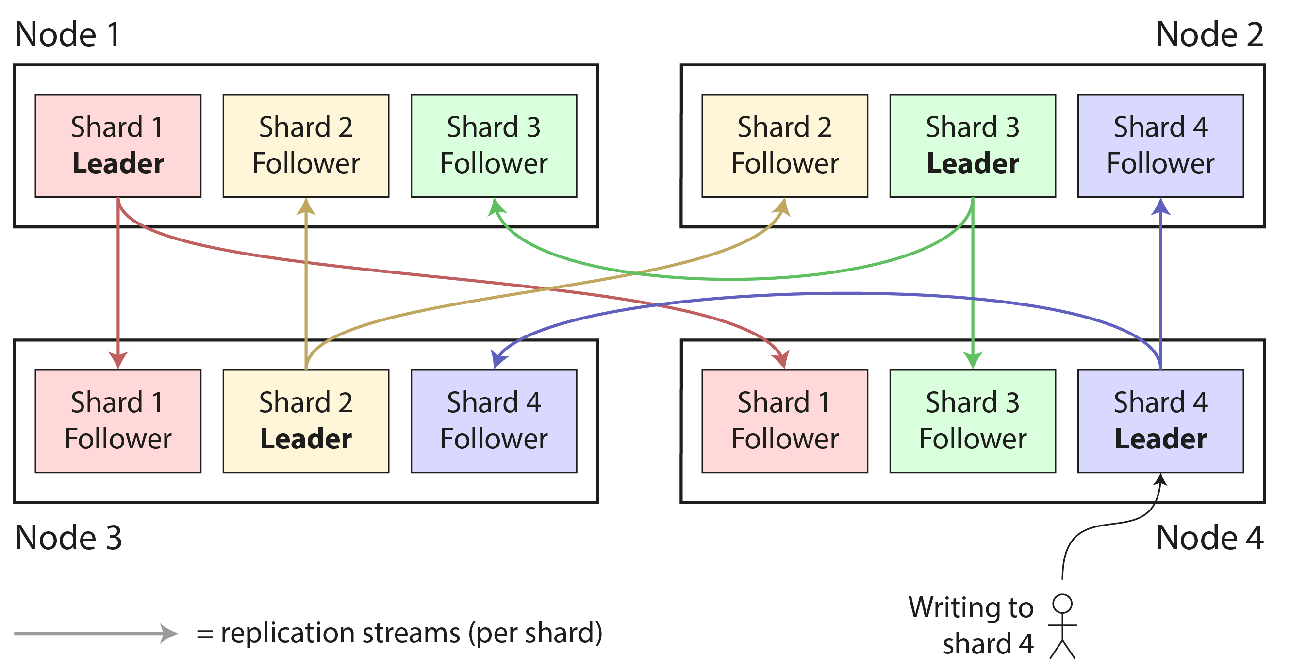
Figure 7-1 Combining replication and sharding: each node acts as leader for some shards and follower for other shards.

Everything we discussed in Chapter 6 about replication of databases applies equally to replication of shards. Since the choice of sharding scheme is mostly independent of the choice of replication scheme, we will ignore replication in this chapter for the sake of simplicity.

SHARDING AND PARTITIONING

What we call a shard in this chapter has many different names depending on which software you’re using: it’s called a partition in Kafka, a range in CockroachDB, a region in HBase and TiDB, a tablet in Bigtable and YugabyteDB, a vnode in Cassandra, ScyllaDB, and Riak, and a vBucket in Couchbase, to name just a few.

Some databases treat partitions and shards as two distinct concepts. For example, in PostgreSQL, partitioning is a way of splitting a large table into several files that are stored on the same machine (which has several advantages, such as making it very fast to delete an entire partition), whereas sharding splits a dataset across multiple machines ¹ ². In many other systems, partitioning is just another word for sharding.

While partitioning is quite descriptive, the term sharding is perhaps surprising. According to one theory, the term arose from the online role-play game Ultima Online, in which a magic crystal was shattered into pieces, and each of those shards refracted a copy of the game world ³. The term shard thus came to mean one of a set of parallel game servers, and later was carried over to databases. Another theory is that shard was originally an acronym of System for Highly Available Replicated Data—reportedly a 1980s database, details of which are lost to history.

By the way, partitioning has nothing to do with network partitions (netsplits), a type of fault in the network between nodes. We will discuss such faults in Chapter 9.

Pros and Cons of Sharding

The primary reason for sharding a database is scalability: it’s a solution if the volume of data or the write throughput has become too great for a single node to handle, as it allows you to spread that data and those writes across multiple nodes. (If read throughput is the problem, you don’t necessarily need sharding—you can use read scaling as discussed in Chapter 6.)

In fact, sharding is one of the main tools we have for achieving horizontal scaling (a scale-out architecture), as discussed in “Shared-Memory, Shared-Disk, and Shared-Nothing Architecture”: that is, allowing a system to grow its capacity not by moving to a bigger machine, but by adding more (smaller) machines. If you can divide the workload such that each shard handles a roughly equal share, you can then assign those shards to different machines in order to process their data and queries in parallel.

While replication is useful at both small and large scale, because it enables fault tolerance and offline operation, sharding is a heavyweight solution that is mostly relevant at large scale. If your data volume and write throughput are such that you can process them on a single machine (and a single machine can do a lot nowadays!), it’s often better to avoid sharding and stick with a single-shard database.

The reason for this recommendation is that sharding often adds complexity: you typically have to decide which records to put in which shard by choosing a partition key; all records with the same partition key are placed in the same shard ⁴. This choice matters because accessing a record is fast if you know which shard it’s in, but if you don’t know the shard you have to do an inefficient search across all shards, and the sharding scheme is difficult to change.

Thus, sharding often works well for key-value data, where you can easily shard by key, but it’s harder with relational data where you may want to search by a secondary index, or join records that may be distributed across different shards. We will discuss this further in “Sharding and Secondary Indexes”.

Another problem with sharding is that a write may need to update related records in several different shards. While transactions on a single node are quite common (see Chapter 8), ensuring consistency across multiple shards requires a distributed transaction. As we shall see in Chapter 8, distributed transactions are available in some databases, but they are usually much slower than single-node transactions, may become a bottleneck for the system as a whole, and some systems don’t support them at all.

Some systems use sharding even on a single machine, typically running one single-threaded process per CPU core to make use of the parallelism in the CPU, or to take advantage of a nonuniform memory access (NUMA) architecture in which some banks of memory are closer to one CPU than to others ⁵. For example, Redis, VoltDB, and FoundationDB use one process per core, and rely on sharding to spread load across CPU cores in the same machine ⁶.

Sharding for Multitenancy

Software as a Service (SaaS) products and cloud services are often multitenant, where each tenant is a customer. Multiple users may have logins on the same tenant, but each tenant has a self-contained dataset that is separate from other tenants. For example, in an email marketing service, each business that signs up is typically a separate tenant, since one business’s newsletter signups, delivery data etc. are separate from those of other businesses.

Sometimes sharding is used to implement multitenant systems: either each tenant is given a separate shard, or multiple small tenants may be grouped together into a larger shard. These shards might be physically separate databases (which we previously touched on in “Embedded storage engines”), or separately manageable portions of a larger logical database ⁷. Using sharding for multitenancy has several advantages:

Resource isolation: If one tenant performs a computationally expensive operation, it is less likely that other tenants’ performance will be affected if they are running on different shards.
Permission isolation: If there is a bug in your access control logic, it’s less likely that you will accidentally give one tenant access to another tenant’s data if those tenants’ datasets are stored physically separately from each other.
Cell-based architecture: You can apply sharding not only at the data storage level, but also for the services running your application code. In a cell-based architecture, the services and storage for a particular set of tenants are grouped into a self-contained cell, and different cells are set up such that they can run largely independently from each other. This approach provides fault isolation: that is, a fault in one cell remains limited to that cell, and tenants in other cells are not affected ⁸.
Per-tenant backup and restore: Backing up each tenant’s shard separately makes it possible to restore a tenant’s state from a backup without affecting other tenants, which can be useful in case the tenant accidentally deletes or overwrites important data ⁹.
Regulatory compliance: Data privacy regulation such as the GDPR gives individuals the right to access and delete all data stored about them. If each person’s data is stored in a separate shard, this translates into simple data export and deletion operations on their shard ¹⁰.
Data residence: If a particular tenant’s data needs to be stored in a particular jurisdiction in order to comply with data residency laws, a region-aware database can allow you to assign that tenant’s shard to a particular region.
Gradual schema rollout: Schema migrations (previously discussed in “Schema flexibility in the document model”) can be rolled out gradually, one tenant at a time. This reduces risk, as you can detect problems before they affect all tenants, but it can be difficult to do transactionally ¹¹.

The main challenges around using sharding for multitenancy are:

It assumes that each individual tenant is small enough to fit on a single node. If that is not the case, and you have a single tenant that’s too big for one machine, you would need to additionally perform sharding within a single tenant, which brings us back to the topic of sharding for scalability ¹².
If you have many small tenants, then creating a separate shard for each one may incur too much overhead. You could group several small tenants together into a bigger shard, but then you have the problem of how you move tenants from one shard to another as they grow.
If you ever need to support features that connect data across multiple tenants, these become harder to implement if you need to join data across multiple shards.

Sharding of Key-Value Data

Say you have a large amount of data, and you want to shard it. How do you decide which records to store on which nodes?

Our goal with sharding is to spread the data and the query load evenly across nodes. If every node takes a fair share, then—in theory—10 nodes should be able to handle 10 times as much data and 10 times the read and write throughput of a single node (ignoring replication). Moreover, if we add or remove a node, we want to be able to rebalance the load so that it is evenly distributed across the 11 (when adding) or the remaining 9 (when removing) nodes.

If the sharding is unfair, so that some shards have more data or queries than others, we call it skewed. The presence of skew makes sharding much less effective. In an extreme case, all the load could end up on one shard, so 9 out of 10 nodes are idle and your bottleneck is the single busy node. A shard with disproportionately high load is called a hot shard or hot spot. If there’s one key with a particularly high load (e.g., a celebrity in a social network), we call it a hot key.

Therefore we need an algorithm that takes as input the partition key of a record, and tells us which shard that record is in. In a key-value store the partition key is usually the key, or the first part of the key. In a relational model the partition key might be some column of a table (not necessarily its primary key). That algorithm needs to be amenable to rebalancing in order to relieve hot spots.

Sharding by Key Range

One way of sharding is to assign a contiguous range of partition keys (from some minimum to some maximum) to each shard, like the volumes of a paper encyclopedia, as illustrated in Figure 7-2. In this example, an entry’s partition key is its title. If you want to look up the entry for a particular title, you can easily determine which shard contains that entry by finding the volume whose key range contains the title you’re looking for, and thus pick the correct book off the shelf.

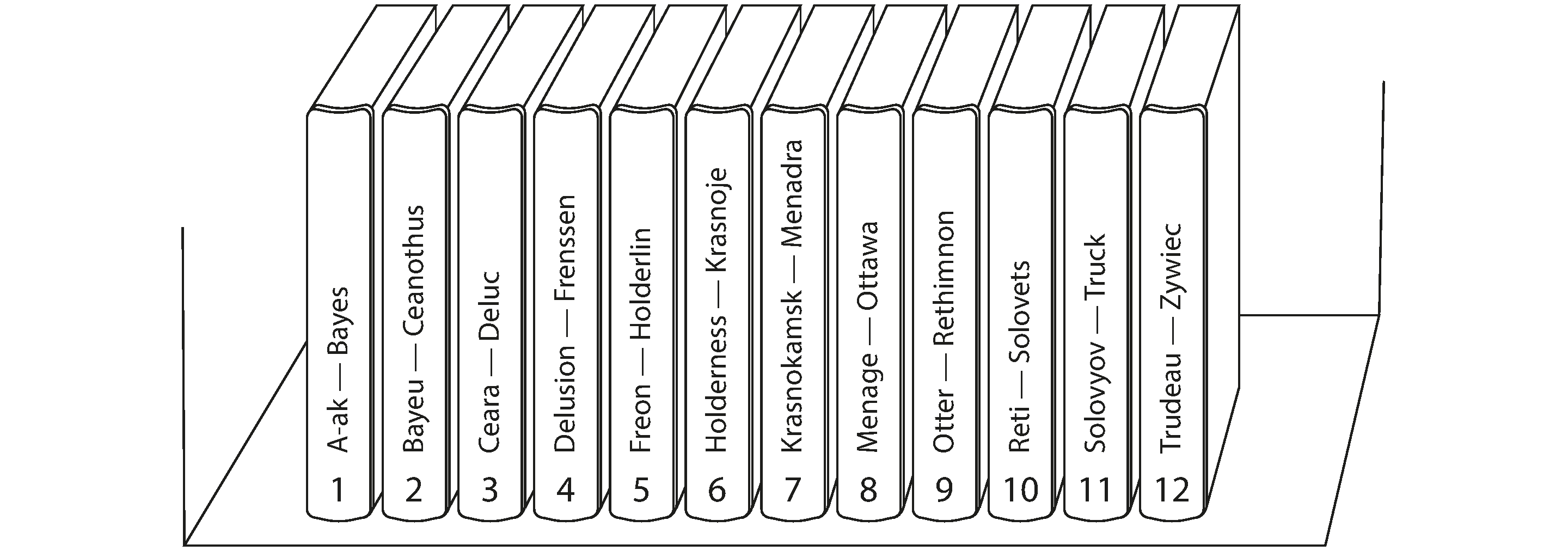
Figure 7-2 A print encyclopedia is sharded by key range.

The ranges of keys are not necessarily evenly spaced, because your data may not be evenly distributed. For example, in Figure 7-2, volume 1 contains words starting with A and B, but volume 12 contains words starting with T, U, V, W, X, Y, and Z. Simply having one volume per two letters of the alphabet would lead to some volumes being much bigger than others. In order to distribute the data evenly, the shard boundaries need to adapt to the data.

The shard boundaries might be chosen manually by an administrator, or the database can choose them automatically. Manual key-range sharding is used by Vitess (a sharding layer for MySQL), for example; the automatic variant is used by Bigtable, its open source equivalent HBase, the range-based sharding option in MongoDB, CockroachDB, RethinkDB, and FoundationDB ⁶. YugabyteDB offers both manual and automatic tablet splitting.

Within each shard, keys are stored in sorted order (e.g., in a B-tree or SSTables, as discussed in Chapter 4). This has the advantage that range scans are easy, and you can treat the key as a concatenated index in order to fetch several related records in one query (see “Multidimensional and Full-Text Indexes”). For example, consider an application that stores data from a network of sensors, where the key is the timestamp of the measurement. Range scans are very useful in this case, because they let you easily fetch, say, all the readings from a particular month.

A downside of key range sharding is that you can easily get a hot shard if there are a lot of writes to nearby keys. For example, if the key is a timestamp, then the shards correspond to ranges of time—e.g., one shard per month. Unfortunately, if you write data from the sensors to the database as the measurements happen, all the writes end up going to the same shard (the one for this month), so that shard can be overloaded with writes while others sit idle ¹³.

To avoid this problem in the sensor database, you need to use something other than the timestamp as the first element of the key. For example, you could prefix each timestamp with the sensor ID so that the key ordering is first by sensor ID and then by timestamp. Assuming you have many sensors active at the same time, the write load will end up more evenly spread across the shards. The downside is that when you want to fetch the values of multiple sensors within a time range, you now need to perform a separate range query for each sensor.

Rebalancing key-range sharded data

When you first set up your database, there are no key ranges to split into shards. Some databases, such as HBase and MongoDB, allow you to configure an initial set of shards on an empty database, which is called pre-splitting. This requires that you already have some idea of what the key distribution is going to look like, so that you can choose appropriate key range boundaries ¹⁴.

Later on, as your data volume and write throughput grow, a system with key-range sharding grows by splitting an existing shard into two or more smaller shards, each of which holds a contiguous sub-range of the original shard’s key range. The resulting smaller shards can then be distributed across multiple nodes. If large amounts of data are deleted, you may also need to merge several adjacent shards that have become small into one bigger one. This process is similar to what happens at the top level of a B-tree (see “B-Trees”).

With databases that manage shard boundaries automatically, a shard split is typically triggered by:

the shard reaching a configured size (for example, on HBase, the default is 10 GB), or
in some systems, the write throughput being persistently above some threshold. Thus, a hot shard may be split even if it is not storing a lot of data, so that its write load can be distributed more uniformly.

An advantage of key-range sharding is that the number of shards adapts to the data volume. If there is only a small amount of data, a small number of shards is sufficient, so overheads are small; if there is a huge amount of data, the size of each individual shard is limited to a configurable maximum ¹⁵.

A downside of this approach is that splitting a shard is an expensive operation, since it requires all of its data to be rewritten into new files, similarly to a compaction in a log-structured storage engine. A shard that needs splitting is often also one that is under high load, and the cost of splitting can exacerbate that load, risking it becoming overloaded.

Sharding by Hash of Key

Key-range sharding is useful if you want records with nearby (but different) partition keys to be grouped into the same shard; for example, this might be the case with timestamps. If you don’t care whether partition keys are near each other (e.g., if they are tenant IDs in a multitenant application), a common approach is to first hash the partition key before mapping it to a shard.

A good hash function takes skewed data and makes it uniformly distributed. Say you have a 32-bit hash function that takes a string. Whenever you give it a new string, it returns a seemingly random number between 0 and 2³² − 1. Even if the input strings are very similar, their hashes are evenly distributed across that range of numbers (but the same input always produces the same output).

For sharding purposes, the hash function need not be cryptographically strong: for example, MongoDB uses MD5, whereas Cassandra and ScyllaDB use Murmur3. Many programming languages have simple hash functions built in (as they are used for hash tables), but they may not be suitable for sharding: for example, in Java’s Object.hashCode() and Ruby’s Object#hash, the same key may have a different hash value in different processes, making them unsuitable for sharding ¹⁶.

Hash modulo number of nodes

Once you have hashed the key, how do you choose which shard to store it in? Maybe your first thought is to take the hash value modulo the number of nodes in the system (using the % operator in many programming languages). For example, hash(key) % 10 would return a number between 0 and 9 (if we write the hash as a decimal number, the hash % 10 would be the last digit). If we have 10 nodes, numbered 0 to 9, that seems like an easy way of assigning each key to a node.

The problem with the mod N approach is that if the number of nodes N changes, most of the keys have to be moved from one node to another. Figure 7-3 shows what happens when you have three nodes and add a fourth. Before the rebalancing, node 0 stored the keys whose hashes are 0, 3, 6, 9, and so on. After adding the fourth node, the key with hash 3 has moved to node 3, the key with hash 6 has moved to node 2, the key with hash 9 has moved to node 1, and so on.

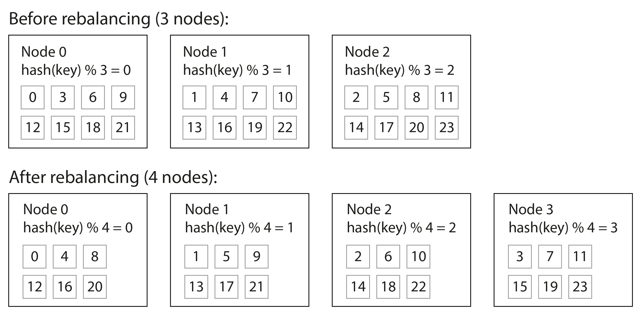
Figure 7-3 Assigning keys to nodes by hashing the key and taking it modulo the number of nodes. Changing the number of nodes results in many keys moving from one node to another.

The mod N function is easy to compute, but it leads to very inefficient rebalancing because there is a lot of unnecessary movement of records from one node to another. We need an approach that doesn’t move data around more than necessary.

Fixed number of shards

One simple but widely-used solution is to create many more shards than there are nodes, and to assign several shards to each node. For example, a database running on a cluster of 10 nodes may be split into 1,000 shards from the outset so that 100 shards are assigned to each node. A key is then stored in shard number hash(key) % 1,000, and the system separately keeps track of which shard is stored on which node.

Now, if a node is added to the cluster, the system can reassign some of the shards from existing nodes to the new node until they are fairly distributed once again. This process is illustrated in Figure 7-4. If a node is removed from the cluster, the same happens in reverse.

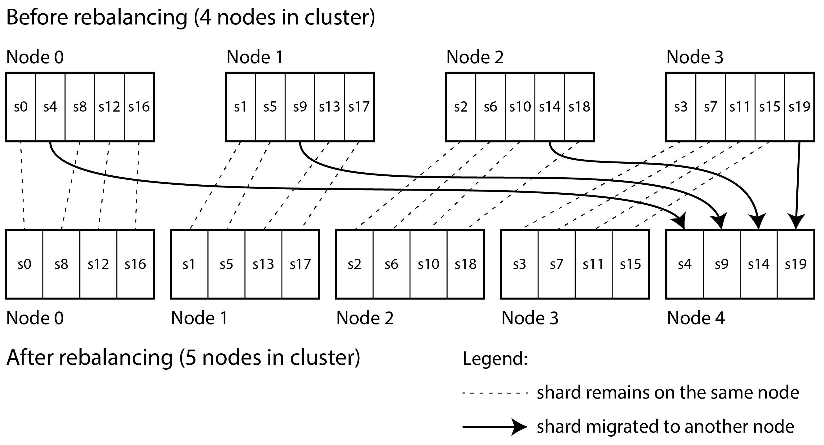
Figure 7-4 Adding a new node to a database cluster with multiple shards per node.

In this model, only entire shards are moved between nodes, which is cheaper than splitting shards. The number of shards does not change, nor does the assignment of keys to shards. The only thing that changes is the assignment of shards to nodes. This change of assignment is not immediate—it takes some time to transfer a large amount of data over the network—so the old assignment of shards is used for any reads and writes that happen while the transfer is in progress.

It’s common to choose the number of shards to be a number that is divisible by many factors, so that the dataset can be evenly split across various different numbers of nodes—not requiring the number of nodes to be a power of 2, for example ⁴. You can even account for mismatched hardware in your cluster: by assigning more shards to nodes that are more powerful, you can make those nodes take a greater share of the load.

This approach to sharding is used in Citus (a sharding layer for PostgreSQL), Riak, Elasticsearch, and Couchbase, among others. It works well as long as you have a good estimate of how many shards you will need when you first create the database. You can then add or remove nodes easily, subject to the limitation that you can’t have more nodes than you have shards.

If you find the originally configured number of shards to be wrong—for example, if you have reached a scale where you need more nodes than you have shards—then an expensive resharding operation is required. It needs to split each shard and write it out to new files, using a lot of additional disk space in the process. Some systems don’t allow resharding while concurrently writing to the database, which makes it difficult to change the number of shards without downtime.

Choosing the right number of shards is difficult if the total size of the dataset is highly variable (for example, if it starts small but may grow much larger over time). Since each shard contains a fixed fraction of the total data, the size of each shard grows proportionally to the total amount of data in the cluster. If shards are very large, rebalancing and recovery from node failures become expensive. But if shards are too small, they incur too much overhead. The best performance is achieved when the size of shards is “just right,” neither too big nor too small, which can be hard to achieve if the number of shards is fixed but the dataset size varies.

Sharding by hash range

If the required number of shards can’t be predicted in advance, it’s better to use a scheme in which the number of shards can adapt easily to the workload. The aforementioned key-range sharding scheme has this property, but it has a risk of hot spots when there are a lot of writes to nearby keys. One solution is to combine key-range sharding with a hash function so that each shard contains a range of hash values rather than a range of keys.

Figure 7-5 shows an example using a 16-bit hash function that returns a number between 0 and 65,535 = 2¹⁶ − 1 (in reality, the hash is usually 32 bits or more). Even if the input keys are very similar (e.g., consecutive timestamps), their hashes are uniformly distributed across that range. We can then assign a range of hash values to each shard: for example, values between 0 and 16,383 to shard 0, values between 16,384 and 32,767 to shard 1, and so on.

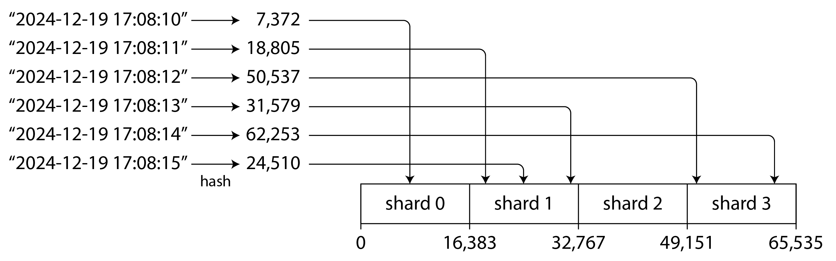
Figure 7-5 Assigning a contiguous range of hash values to each shard.

Like with key-range sharding, a shard in hash-range sharding can be split when it becomes too big or too heavily loaded. This is still an expensive operation, but it can happen as needed, so the number of shards adapts to the volume of data rather than being fixed in advance.

The downside compared to key-range sharding is that range queries over the partition key are not efficient, as keys in the range are now scattered across all the shards. However, if keys consist of two or more columns, and the partition key is only the first of these columns, you can still perform efficient range queries over the second and later columns: as long as all records in the range query have the same partition key, they will be in the same shard.

PARTITIONING AND RANGE QUERIES IN DATA WAREHOUSES

Data warehouses such as BigQuery, Snowflake, and Delta Lake support a similar indexing approach, though the terminology differs. In BigQuery, for example, the partition key determines which partition a record resides in while “cluster columns” determine how records are sorted within the partition. Snowflake assigns records to “micro-partitions” automatically, but allows users to define cluster keys for a table. Delta Lake supports both manual and automatic partition assignment, and supports cluster keys. Clustering data not only improves range scan performance, but can improve compression and filtering performance as well.

Hash-range sharding is used in YugabyteDB and DynamoDB ¹⁷, and is an option in MongoDB. Cassandra and ScyllaDB use a variant of this approach that is illustrated in Figure 7-6: the space of hash values is split into a number of ranges proportional to the number of nodes (3 ranges per node in Figure 7-6, but actual numbers are 8 per node in Cassandra by default, and 256 per node in ScyllaDB), with random boundaries between those ranges. This means some ranges are bigger than others, but by having multiple ranges per node those imbalances tend to even out ¹⁵ ¹⁸.

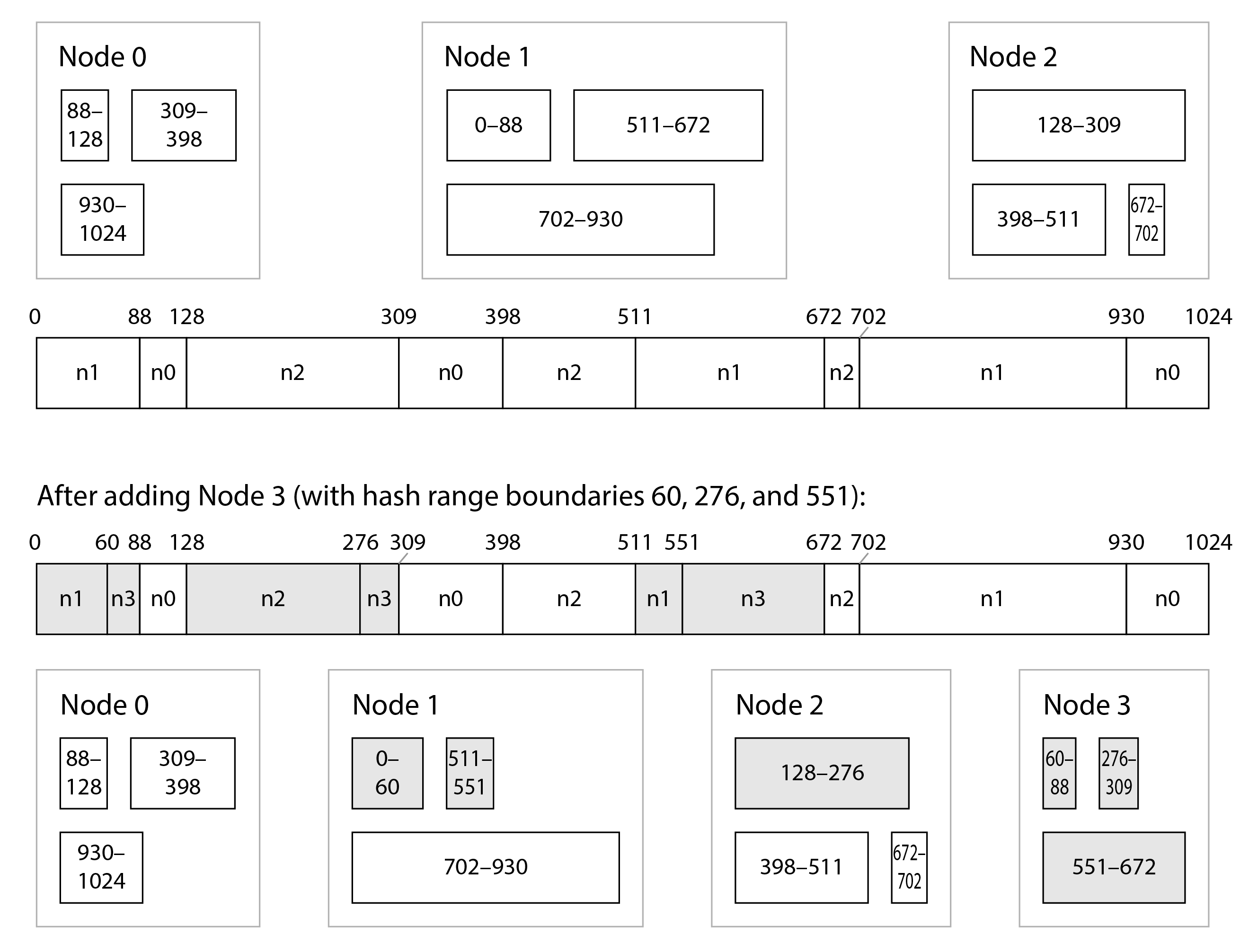
Figure 7-6 Cassandra and ScyllaDB split the range of possible hash values (here 0–1023) into contiguous ranges with random boundaries, and assign several ranges to each node.

When nodes are added or removed, range boundaries are added and removed, and shards are split or merged accordingly ¹⁹. In the example of Figure 7-6, when node 3 is added, node 1 transfers parts of two of its ranges to node 3, and node 2 transfers part of one of its ranges to node 3. This has the effect of giving the new node an approximately fair share of the dataset, without transferring more data than necessary from one node to another.

Consistent hashing

A consistent hashing algorithm is a hash function that maps keys to a specified number of shards in a way that satisfies two properties:

the number of keys mapped to each shard is roughly equal, and
when the number of shards changes, as few keys as possible are moved from one shard to another.

Note that consistent here has nothing to do with replica consistency (see Chapter 6) or ACID consistency (see Chapter 8), but rather describes the tendency of a key to stay in the same shard as much as possible.

The sharding algorithm used by Cassandra and ScyllaDB is similar to the original definition of consistent hashing ²⁰, but several other consistent hashing algorithms have also been proposed ²¹, such as highest random weight, also known as rendezvous hashing ²², and jump consistent hash ²³. With Cassandra’s algorithm, if one node is added, a small number of existing shards are split into sub-ranges; on the other hand, with rendezvous and jump consistent hashes, the new node is assigned individual keys that were previously scattered across all of the other nodes. Which one is preferable depends on the application.

Skewed Workloads and Relieving Hot Spots

Consistent hashing ensures that keys are uniformly distributed across nodes, but that doesn’t mean that the actual load is uniformly distributed. If the workload is highly skewed—that is, the amount of data under some partition keys is much greater than other keys, or if the rate of requests to some keys is much higher than to others—you can still end up with some servers being overloaded while others sit almost idle.

For example, on a social media site, a celebrity user with millions of followers may cause a storm of activity when they do something ²⁴. This event can result in a large volume of reads and writes to the same key (where the partition key is perhaps the user ID of the celebrity, or the ID of the action that people are commenting on).

In such situations, a more flexible sharding policy is required ²⁵ ²⁶. A system that defines shards based on ranges of keys (or ranges of hashes) makes it possible to put an individual hot key in a shard by its own, and perhaps even assigning it a dedicated machine ²⁷.

It’s also possible to compensate for skew at the application level. For example, if one key is known to be very hot, a simple technique is to add a random number to the beginning or end of the key. Just a two-digit decimal random number would split the writes to the key evenly across 100 different keys, allowing those keys to be distributed to different shards.

However, having split the writes across different keys, any reads now have to do additional work, as they have to read the data from all 100 keys and combine it. The volume of reads to each shard of the hot key is not reduced; only the write load is split. This technique also requires additional bookkeeping: it only makes sense to append the random number for the small number of hot keys; for the vast majority of keys with low write throughput this would be unnecessary overhead. Thus, you also need some way of keeping track of which keys are being split, and a process for converting a regular key into a specially-managed hot key.

The problem is further compounded by change of load over time: for example, a particular social media post that has gone viral may experience high load for a couple of days, but thereafter it’s likely to calm down again. Moreover, some keys may be hot for writes while others are hot for reads, necessitating different strategies for handling them.

Some systems (especially cloud services designed for large scale) have automated approaches for dealing with hot shards; for example, Amazon calls it heat management ²⁸ or adaptive capacity ¹⁷. The details of how these systems work go beyond the scope of this book.

Operations: Automatic or Manual Rebalancing

There is one important question with regard to rebalancing that we have glossed over: does the splitting of shards and rebalancing happen automatically or manually?

Some systems automatically decide when to split shards and when to move them from one node to another, without any human interaction, while others leave sharding to be explicitly configured by an administrator. There is also a middle ground: for example, Couchbase and Riak generate a suggested shard assignment automatically, but require an administrator to commit it before it takes effect.

Fully automated rebalancing can be convenient, because there is less operational work to do for normal maintenance, and such systems can even auto-scale to adapt to changes in workload. Cloud databases such as DynamoDB are promoted as being able to automatically add and remove shards to adapt to big increases or decreases of load within a matter of minutes ¹⁷ ²⁹.

However, automatic shard management can also be unpredictable. Rebalancing is an expensive operation, because it requires rerouting requests and moving a large amount of data from one node to another. If it is not done carefully, this process can overload the network or the nodes, and it might harm the performance of other requests. The system must continue processing writes while the rebalancing is in progress; if a system is near its maximum write throughput, the shard-splitting process might not even be able to keep up with the rate of incoming writes ²⁹.

Such automation can be dangerous in combination with automatic failure detection. For example, say one node is overloaded and is temporarily slow to respond to requests. The other nodes conclude that the overloaded node is dead, and automatically rebalance the cluster to move load away from it. This puts additional load on other nodes and the network, making the situation worse. There is a risk of causing a cascading failure where other nodes become overloaded and are also falsely suspected of being down.

For that reason, it can be a good thing to have a human in the loop for rebalancing. It’s slower than a fully automatic process, but it can help prevent operational surprises.

Request Routing

We have discussed how to shard a dataset across multiple nodes, and how to rebalance those shards as nodes are added or removed. Now let’s move on to the question: if you want to read or write a particular key, how do you know which node—i.e., which IP address and port number—you need to connect to?

We call this problem request routing, and it’s very similar to service discovery, which we previously discussed in “Load balancers, service discovery, and service meshes”. The biggest difference between the two is that with services running application code, each instance is usually stateless, and a load balancer can send a request to any of the instances. With sharded databases, a request for a key can only be handled by a node that is a replica for the shard containing that key.

This means that request routing has to be aware of the assignment from keys to shards, and from shards to nodes. On a high level, there are a few different approaches to this problem (illustrated in Figure 7-7):

Allow clients to contact any node (e.g., via a round-robin load balancer). If that node coincidentally owns the shard to which the request applies, it can handle the request directly; otherwise, it forwards the request to the appropriate node, receives the reply, and passes the reply along to the client.
Send all requests from clients to a routing tier first, which determines the node that should handle each request and forwards it accordingly. This routing tier does not itself handle any requests; it only acts as a shard-aware load balancer.
Require that clients be aware of the sharding and the assignment of shards to nodes. In this case, a client can connect directly to the appropriate node, without any intermediary.

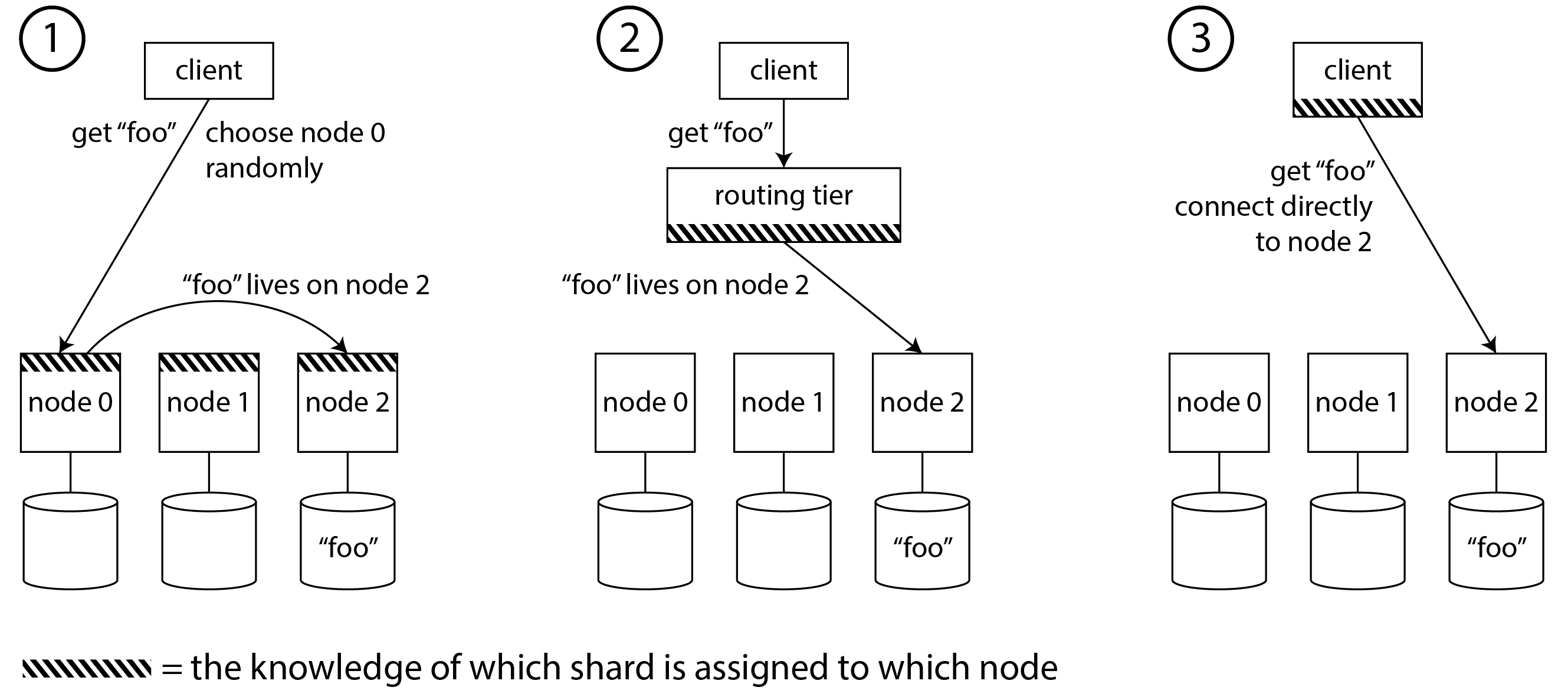
Figure 7-7 Three different ways of routing a request to the right node.

In all cases, there are some key problems:

Who decides which shard should live on which node? It’s simplest to have a single coordinator making that decision, but in that case how do you make it fault-tolerant in case the node running the coordinator goes down? And if the coordinator role can failover to another node, how do you prevent a split-brain situation (see “Handling Node Outages”) where two different coordinators make contradictory shard assignments?
How does the component performing the routing (which may be one of the nodes, or the routing tier, or the client) learn about changes in the assignment of shards to nodes?
While a shard is being moved from one node to another, there is a cutover period during which the new node has taken over, but requests to the old node may still be in flight. How do you handle those?

Many distributed data systems rely on a separate coordination service such as ZooKeeper or etcd to keep track of shard assignments, as illustrated in Figure 7-8. They use consensus algorithms (see Chapter 10) to provide fault tolerance and protection against split-brain. Each node registers itself in ZooKeeper, and ZooKeeper maintains the authoritative mapping of shards to nodes. Other actors, such as the routing tier or the sharding-aware client, can subscribe to this information in ZooKeeper. Whenever a shard changes ownership, or a node is added or removed, ZooKeeper notifies the routing tier so that it can keep its routing information up to date.

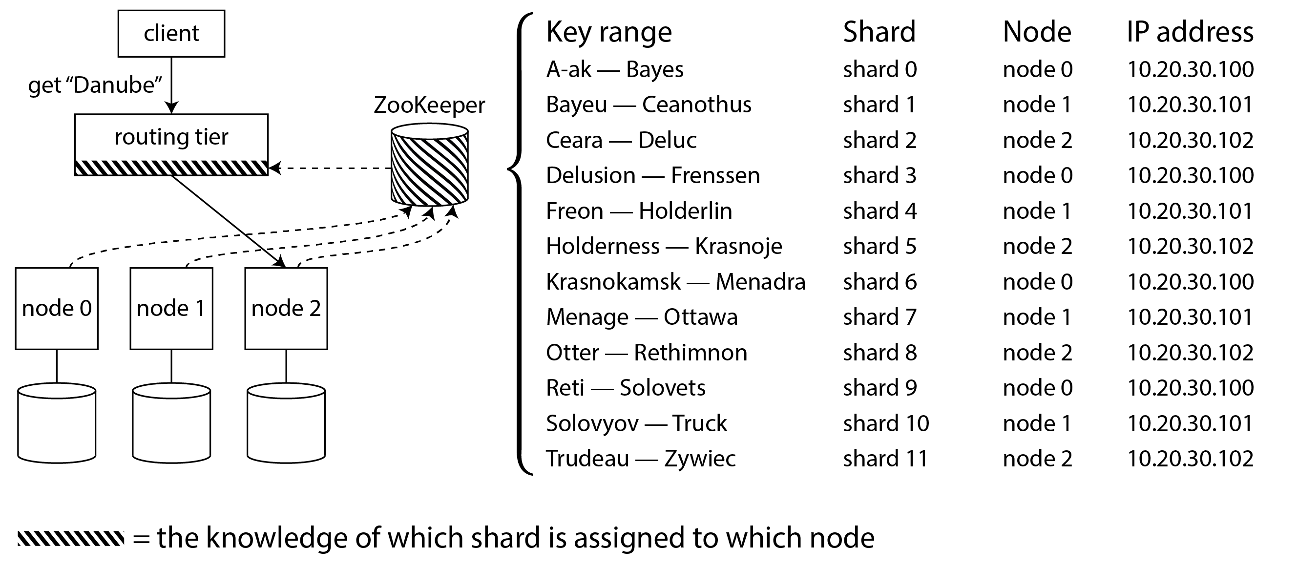
Figure 7-8 Using ZooKeeper to keep track of assignment of shards to nodes.

For example, HBase and SolrCloud use ZooKeeper to manage shard assignment, and Kubernetes uses etcd to keep track of which service instance is running where. MongoDB has a similar architecture, but it relies on its own config server implementation and mongos daemons as the routing tier. Kafka, YugabyteDB, and TiDB use built-in implementations of the Raft consensus protocol to perform this coordination function.

Cassandra, ScyllaDB, and Riak take a different approach: they use a gossip protocol among the nodes to disseminate any changes in cluster state. This provides much weaker consistency than a consensus protocol; it is possible to have split brain, in which different parts of the cluster have different node assignments for the same shard. Leaderless databases can tolerate this because they generally make weak consistency guarantees anyway (see “Limitations of Quorum Consistency”).

When using a routing tier or when sending requests to a random node, clients still need to find the IP addresses to connect to. These are not as fast-changing as the assignment of shards to nodes, so it is often sufficient to use DNS for this purpose.

This discussion of request routing has focused on finding the shard for an individual key, which is most relevant for sharded OLTP databases. Analytic databases often use sharding as well, but they typically have a very different kind of query execution: rather than executing in a single shard, a query typically needs to aggregate and join data from many different shards in parallel. We will discuss techniques for such parallel query execution in “JOIN and GROUP BY”.

Sharding and Secondary Indexes

The sharding schemes we have discussed so far rely on the client knowing the partition key for any record it wants to access. This is most easily done in a key-value data model, where the partition key is the first part of the primary key (or the entire primary key), and so we can use the partition key to determine the shard, and thus route reads and writes to the node that is responsible for that key.

The situation becomes more complicated if secondary indexes are involved (see also “Multi-Column and Secondary Indexes”). A secondary index usually doesn’t identify a record uniquely but rather is a way of searching for occurrences of a particular value: find all actions by user 123, find all articles containing the word hogwash, find all cars whose color is red, and so on.

Key-value stores often don’t have secondary indexes, but they are the bread and butter of relational databases, they are common in document databases too, and they are the raison d’être of full-text search engines such as Solr and Elasticsearch. The problem with secondary indexes is that they don’t map neatly to shards. There are two main approaches to sharding a database with secondary indexes: local and global indexes.

Local Secondary Indexes

For example, imagine you are operating a website for selling used cars (illustrated in Figure 7-9). Each listing has a unique ID, and you use that ID as partition key for sharding (for example, IDs 0 to 499 in shard 0, IDs 500 to 999 in shard 1, etc.).

If you want to let users search for cars, allowing them to filter by color and by make, you need a secondary index on color and make (in a document database these would be fields; in a relational database they would be columns). If you have declared the index, the database can perform the indexing automatically. For example, whenever a red car is added to the database, the database shard automatically adds its ID to the list of IDs for the index entry color:red. As discussed in Chapter 4, that list of IDs is also called a postings list.

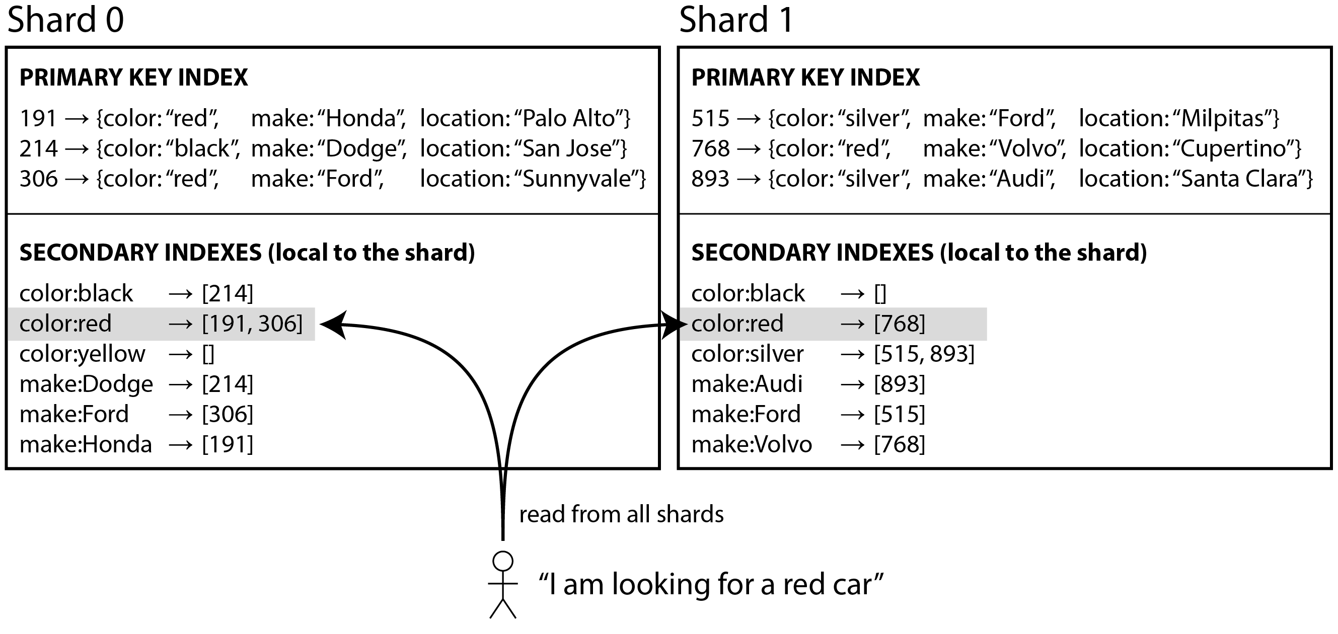
Figure 7-9 Local secondary indexes: each shard indexes only the records within its own shard.

WARNING

If your database only supports a key-value model, you might be tempted to implement a secondary index yourself by creating a mapping from values to IDs in application code. If you go down this route, you need to take great care to ensure your indexes remain consistent with the underlying data. Race conditions and intermittent write failures (where some changes were saved but others weren’t) can very easily cause the data to go out of sync—see “The need for multi-object transactions”.

In this indexing approach, each shard is completely separate: each shard maintains its own secondary indexes, covering only the records in that shard. It doesn’t care what data is stored in other shards. Whenever you write to the database—to add, remove, or update a records—you only need to deal with the shard that contains the record that you are writing. For that reason, this type of secondary index is known as a local index. In an information retrieval context it is also known as a document-partitioned index ³⁰.

When reading from a local secondary index, if you already know the partition key of the record you’re looking for, you can just perform the search on the appropriate shard. Moreover, if you only want some results, and you don’t need all, you can send the request to any shard.

However, if you want all the results and don’t know their partition key in advance, you need to send the query to all shards, and combine the results you get back, because the matching records might be scattered across all the shards. In Figure 7-9, red cars appear in both shard 0 and shard 1.

This approach to querying a sharded database can make read queries on secondary indexes quite expensive. Even if you query the shards in parallel, it is prone to tail latency amplification (see “Use of Response Time Metrics”). It also limits the scalability of your application: adding more shards lets you store more data, but it doesn’t increase your query throughput if every shard has to process every query anyway.

Nevertheless, local secondary indexes are widely used ³¹: for example, MongoDB, Riak, Cassandra ³², Elasticsearch ³³, SolrCloud, and VoltDB ³⁴ all use local secondary indexes.

Global Secondary Indexes

Rather than each shard having its own, local secondary index, we can construct a global index that covers data in all shards. However, we can’t just store that index on one node, since it would likely become a bottleneck and defeat the purpose of sharding. A global index must also be sharded, but it can be sharded differently from the primary key index.

Figure 7-10 illustrates what this could look like: the IDs of red cars from all shards appear under color:red in the index, but the index is sharded so that colors starting with the letters a to r appear in shard 0 and colors starting with s to z appear in shard 1. The index on the make of car is partitioned similarly (with the shard boundary being between f and h).

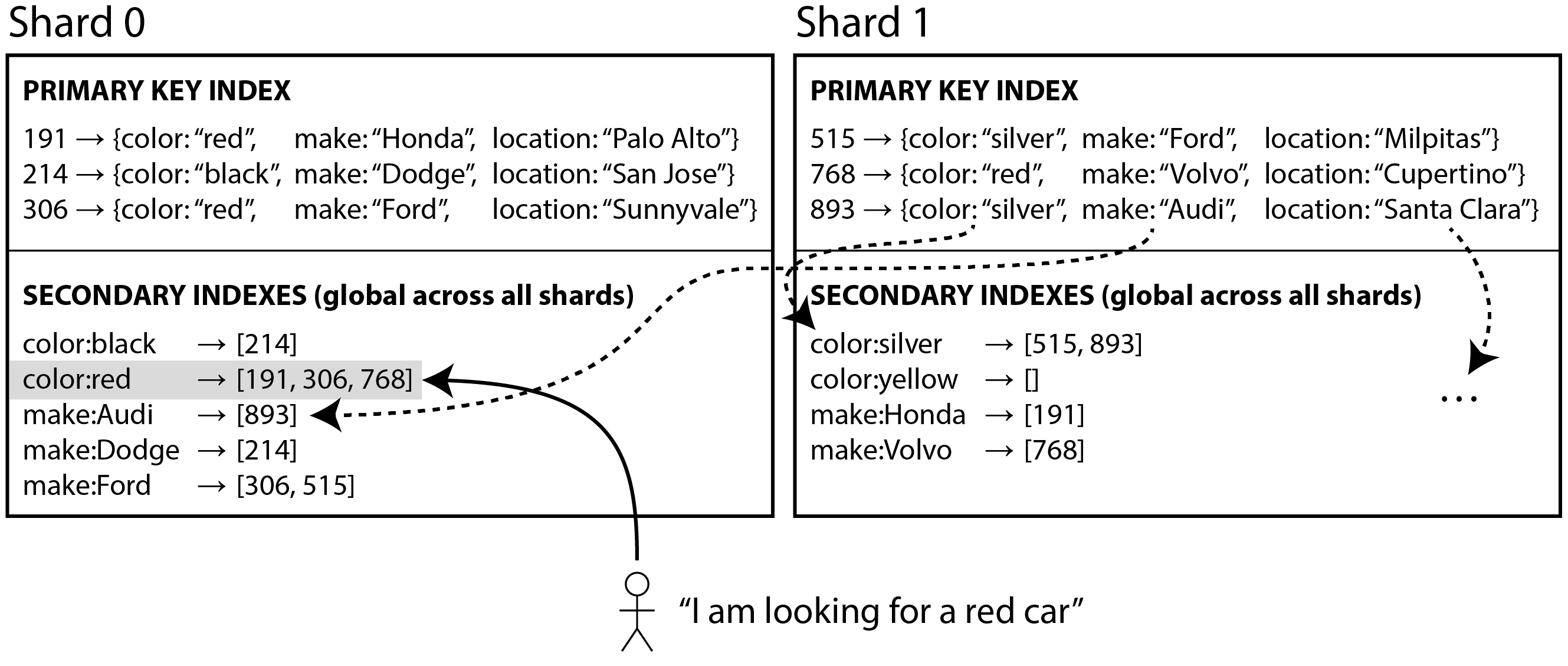
Figure 7-10 A global secondary index reflects data from all shards, and is itself sharded by the indexed value.

This kind of index is also called term-partitioned ³⁰: recall from “Full-Text Search” that in full-text search, a term is a keyword in a text that you can search for. Here we generalise it to mean any value that you can search for in the secondary index.

The global index uses the term as partition key, so that when you’re looking for a particular term or value, you can figure out which shard you need to query. As before, a shard can contain a contiguous range of terms (as in Figure 7-10), or you can assign terms to shards based on a hash of the term.

Global indexes have the advantage that a query with a single condition (such as color = red) only needs to read from a single shard to fetch the postings list. However, if you want to fetch records and not just IDs, you still have to read from all the shards that are responsible for those IDs.

If you have multiple search conditions or terms (e.g., searching for cars of a certain color and a certain make, or searching for multiple words occurring in the same text), it’s likely that those terms will be assigned to different shards. To compute the logical AND of the two conditions, the system needs to find all the IDs that occur in both of the postings lists. That’s no problem if the postings lists are short, but if they are long, it can be slow to send them over the network to compute their intersection ³⁰.

Another challenge with global secondary indexes is that writes are more complicated than with local indexes, because writing a single record might affect multiple shards of the index (every term in the document might be on a different shard). This makes it harder to keep the secondary index in sync with the underlying data. One option is to use a distributed transaction to atomically update the shards storing the primary record and its secondary indexes (see Chapter 8).

Global secondary indexes are used by CockroachDB, TiDB, and YugabyteDB; DynamoDB supports both local and global secondary indexes. In the case of DynamoDB, writes are asynchronously reflected in global indexes, so reads from a global index may be stale (similarly to replication lag, as in “Problems with Replication Lag”). Nevertheless, global indexes are useful if read throughput is higher than write throughput, and if the postings lists are not too long.

Summary

In this chapter we explored different ways of sharding a large dataset into smaller subsets. Sharding is necessary when you have so much data that storing and processing it on a single machine is no longer feasible.

The goal of sharding is to spread the data and query load evenly across multiple machines, avoiding hot spots (nodes with disproportionately high load). This requires choosing a sharding scheme that is appropriate to your data, and rebalancing the shards when nodes are added to or removed from the cluster.

We discussed two main approaches to sharding:

Key range sharding, where keys are sorted, and a shard owns all the keys from some minimum up to some maximum. Sorting has the advantage that efficient range queries are possible, but there is a risk of hot spots if the application often accesses keys that are close together in the sorted order.

In this approach, shards are typically rebalanced by splitting the range into two subranges when a shard gets too big.

Hash sharding, where a hash function is applied to each key, and a shard owns a range of hash values (or another consistent hashing algorithm may be used to map hashes to shards). This method destroys the ordering of keys, making range queries inefficient, but it may distribute load more evenly.

When sharding by hash, it is common to create a fixed number of shards in advance, to assign several shards to each node, and to move entire shards from one node to another when nodes are added or removed. Splitting shards, like with key ranges, is also possible.

It is common to use the first part of the key as the partition key (i.e., to identify the shard), and to sort records within that shard by the rest of the key. That way you can still have efficient range queries among the records with the same partition key.

We also discussed the interaction between sharding and secondary indexes. A secondary index also needs to be sharded, and there are two methods:

Local secondary indexes, where the secondary indexes are stored in the same shard as the primary key and value. This means that only a single shard needs to be updated on write, but a lookup of the secondary index requires reading from all shards.
Global secondary indexes, which are sharded separately based on the indexed values. An entry in the secondary index may refer to records from all shards of the primary key. When a record is written, several secondary index shards may need to be updated; however, a read of the postings list can be served from a single shard (fetching the actual records still requires reading from multiple shards).

Finally, we discussed techniques for routing queries to the appropriate shard, and how a coordination service is often used to keep track of the assigment of shards to nodes.

By design, every shard operates mostly independently—that’s what allows a sharded database to scale to multiple machines. However, operations that need to write to several shards can be problematic: for example, what happens if the write to one shard succeeds, but another fails? We will address that question in the following chapters.

References

Claire Giordano. Understanding partitioning and sharding in Postgres and Citus. citusdata.com, August 2023. Archived at perma.cc/8BTK-8959 ↩︎
Brandur Leach. Partitioning in Postgres, 2022 edition. brandur.org, October 2022. Archived at perma.cc/Z5LE-6AKX ↩︎
Raph Koster. Database “sharding” came from UO? raphkoster.com, January 2009. Archived at perma.cc/4N9U-5KYF ↩︎
Garrett Fidalgo. Herding elephants: Lessons learned from sharding Postgres at Notion. notion.com, October 2021. Archived at perma.cc/5J5V-W2VX ↩︎ ↩︎
Ulrich Drepper. What Every Programmer Should Know About Memory. akkadia.org, November 2007. Archived at perma.cc/NU6Q-DRXZ ↩︎
Jingyu Zhou, Meng Xu, Alexander Shraer, Bala Namasivayam, Alex Miller, Evan Tschannen, Steve Atherton, Andrew J. Beamon, Rusty Sears, John Leach, Dave Rosenthal, Xin Dong, Will Wilson, Ben Collins, David Scherer, Alec Grieser, Young Liu, Alvin Moore, Bhaskar Muppana, Xiaoge Su, and Vishesh Yadav. FoundationDB: A Distributed Unbundled Transactional Key Value Store. At ACM International Conference on Management of Data (SIGMOD), June 2021. doi:10.1145/3448016.3457559 ↩︎ ↩︎
Marco Slot. Citus 12: Schema-based sharding for PostgreSQL. citusdata.com, July 2023. Archived at perma.cc/R874-EC9W ↩︎
Robisson Oliveira. Reducing the Scope of Impact with Cell-Based Architecture. AWS Well-Architected white paper, Amazon Web Services, September 2023. Archived at perma.cc/4KWW-47NR ↩︎
Gwen Shapira. Things DBs Don’t Do - But Should. thenile.dev, February 2023. Archived at perma.cc/C3J4-JSFW ↩︎
Malte Schwarzkopf, Eddie Kohler, M. Frans Kaashoek, and Robert Morris. Position: GDPR Compliance by Construction. At Towards Polystores that manage multiple Databases, Privacy, Security and/or Policy Issues for Heterogenous Data (Poly), August 2019. doi:10.1007/978-3-030-33752-0_3 ↩︎
Gwen Shapira. Introducing pg_karnak: Transactional schema migration across tenant databases. thenile.dev, November 2024. Archived at perma.cc/R5RD-8HR9 ↩︎
Arka Ganguli, Guido Iaquinti, Maggie Zhou, and Rafael Chacón. Scaling Datastores at Slack with Vitess. slack.engineering, December 2020. Archived at perma.cc/UW8F-ALJK ↩︎
Ikai Lan. App Engine Datastore Tip: Monotonically Increasing Values Are Bad. ikaisays.com, January 2011. Archived at perma.cc/BPX8-RPJB ↩︎
Enis Soztutar. Apache HBase Region Splitting and Merging. cloudera.com, February 2013. Archived at perma.cc/S9HS-2X2C ↩︎
Eric Evans. Rethinking Topology in Cassandra. At Cassandra Summit, June 2013. Archived at perma.cc/2DKM-F438 ↩︎ ↩︎
Martin Kleppmann. Java’s hashCode Is Not Safe for Distributed Systems. martin.kleppmann.com, June 2012. Archived at perma.cc/LK5U-VZSN ↩︎
Mostafa Elhemali, Niall Gallagher, Nicholas Gordon, Joseph Idziorek, Richard Krog, Colin Lazier, Erben Mo, Akhilesh Mritunjai, Somu Perianayagam, Tim Rath, Swami Sivasubramanian, James Christopher Sorenson III, Sroaj Sosothikul, Doug Terry, and Akshat Vig. Amazon DynamoDB: A Scalable, Predictably Performant, and Fully Managed NoSQL Database Service. At USENIX Annual Technical Conference (ATC), July 2022. ↩︎ ↩︎ ↩︎
Brandon Williams. Virtual Nodes in Cassandra 1.2. datastax.com, December 2012. Archived at perma.cc/N385-EQXV ↩︎
Branimir Lambov. New Token Allocation Algorithm in Cassandra 3.0. datastax.com, January 2016. Archived at perma.cc/2BG7-LDWY ↩︎
David Karger, Eric Lehman, Tom Leighton, Rina Panigrahy, Matthew Levine, and Daniel Lewin. Consistent Hashing and Random Trees: Distributed Caching Protocols for Relieving Hot Spots on the World Wide Web. At 29th Annual ACM Symposium on Theory of Computing (STOC), May 1997. doi:10.1145/258533.258660 ↩︎
Damian Gryski. Consistent Hashing: Algorithmic Tradeoffs. dgryski.medium.com, April 2018. Archived at perma.cc/B2WF-TYQ8 ↩︎
David G. Thaler and Chinya V. Ravishankar. Using name-based mappings to increase hit rates. IEEE/ACM Transactions on Networking, volume 6, issue 1, pages 1–14, February 1998. doi:10.1109/90.663936 ↩︎
John Lamping and Eric Veach. A Fast, Minimal Memory, Consistent Hash Algorithm. arxiv.org, June 2014. ↩︎
Samuel Axon. 3% of Twitter’s Servers Dedicated to Justin Bieber. mashable.com, September 2010. Archived at perma.cc/F35N-CGVX ↩︎
Gerald Guo and Thawan Kooburat. Scaling services with Shard Manager. engineering.fb.com, August 2020. Archived at perma.cc/EFS3-XQYT ↩︎
Sangmin Lee, Zhenhua Guo, Omer Sunercan, Jun Ying, Thawan Kooburat, Suryadeep Biswal, Jun Chen, Kun Huang, Yatpang Cheung, Yiding Zhou, Kaushik Veeraraghavan, Biren Damani, Pol Mauri Ruiz, Vikas Mehta, and Chunqiang Tang. Shard Manager: A Generic Shard Management Framework for Geo-distributed Applications. 28th ACM SIGOPS Symposium on Operating Systems Principles (SOSP), pages 553–569, October 2021. doi:10.1145/3477132.3483546 ↩︎
Scott Lystig Fritchie. A Critique of Resizable Hash Tables: Riak Core & Random Slicing. infoq.com, August 2018. Archived at perma.cc/RPX7-7BLN ↩︎
Andy Warfield. Building and operating a pretty big storage system called S3. allthingsdistributed.com, July 2023. Archived at perma.cc/6S7P-GLM4 ↩︎
Rich Houlihan. DynamoDB adaptive capacity: smooth performance for chaotic workloads (DAT327). At AWS re:Invent, November 2017. ↩︎ ↩︎
Christopher D. Manning, Prabhakar Raghavan, and Hinrich Schütze. Introduction to Information Retrieval. Cambridge University Press, 2008. ISBN: 978-0-521-86571-5, available online at nlp.stanford.edu/IR-book ↩︎ ↩︎ ↩︎
Michael Busch, Krishna Gade, Brian Larson, Patrick Lok, Samuel Luckenbill, and Jimmy Lin. Earlybird: Real-Time Search at Twitter. At 28th IEEE International Conference on Data Engineering (ICDE), April 2012. doi:10.1109/ICDE.2012.149 ↩︎
Nadav Har’El. Indexing in Cassandra 3. github.com, April 2017. Archived at perma.cc/3ENV-8T9P ↩︎
Zachary Tong. Customizing Your Document Routing. elastic.co, June 2013. Archived at perma.cc/97VM-MREN ↩︎
Andrew Pavlo. H-Store Frequently Asked Questions. hstore.cs.brown.edu, October 2013. Archived at perma.cc/X3ZA-DW6Z ↩︎

8. Transactions

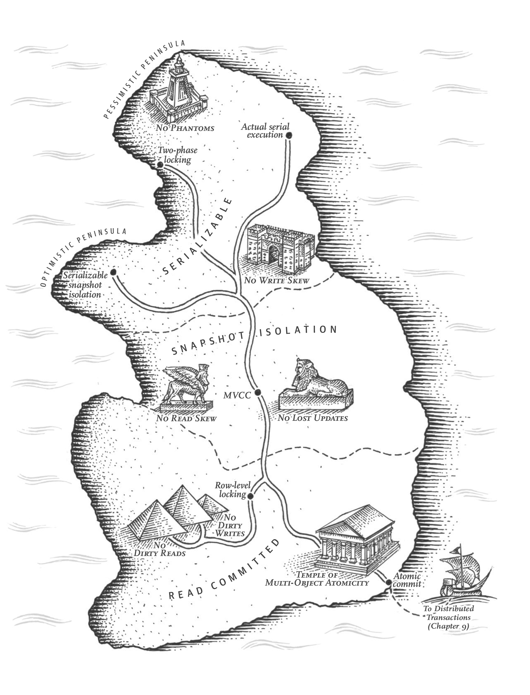
Some authors have claimed that general two-phase commit is too expensive to support, because of the performance or availability problems that it brings. We believe it is better to have application programmers deal with performance problems due to overuse of transactions as bottlenecks arise, rather than always coding around the lack of transactions.

James Corbett et al., Spanner: Google’s Globally-Distributed Database (2012)

In the harsh reality of data systems, many things can go wrong:

The database software or hardware may fail at any time (including in the middle of a write operation).
The application may crash at any time (including halfway through a series of operations).
Interruptions in the network can unexpectedly cut off the application from the database, or one database node from another.
Several clients may write to the database at the same time, overwriting each other’s changes.
A client may read data that doesn’t make sense because it has only partially been updated.
Race conditions between clients can cause surprising bugs.

In order to be reliable, a system has to deal with these faults and ensure that they don’t cause catastrophic failure of the entire system. However, implementing fault-tolerance mechanisms is a lot of work. It requires a lot of careful thinking about all the things that can go wrong, and a lot of testing to ensure that the solution actually works.

For decades, transactions have been the mechanism of choice for simplifying these issues. A transaction is a way for an application to group several reads and writes together into a logical unit. Conceptually, all the reads and writes in a transaction are executed as one operation: either the entire transaction succeeds (commit) or it fails (abort, rollback). If it fails, the application can safely retry. With transactions, error handling becomes much simpler for an application, because it doesn’t need to worry about partial failure—i.e., the case where some operations succeed and some fail (for whatever reason).

If you have spent years working with transactions, they may seem obvious, but we shouldn’t take them for granted. Transactions are not a law of nature; they were created with a purpose, namely to simplify the programming model for applications accessing a database. By using transactions, the application is free to ignore certain potential error scenarios and concurrency issues, because the database takes care of them instead (we call these safety guarantees).

Not every application needs transactions, and sometimes there are advantages to weakening transactional guarantees or abandoning them entirely (for example, to achieve higher performance or higher availability). Some safety properties can be achieved without transactions. On the other hand, transactions can prevent a lot of grief: for example, the technical cause behind the Post Office Horizon scandal (see “How Important Is Reliability?”) was probably a lack of ACID transactions in the underlying accounting system ¹.

How do you figure out whether you need transactions? In order to answer that question, we first need to understand exactly what safety guarantees transactions can provide, and what costs are associated with them. Although transactions seem straightforward at first glance, there are actually many subtle but important details that come into play.

In this chapter, we will examine many examples of things that can go wrong, and explore the algorithms that databases use to guard against those issues. We will go especially deep in the area of concurrency control, discussing various kinds of race conditions that can occur and how databases implement isolation levels such as read committed, snapshot isolation, and serializability.

Concurrency control is relevant for both single-node and distributed databases. Later in this chapter, in “Distributed Transactions”, we will examine the two-phase commit protocol and the challenge of achieving atomicity in a distributed transaction.

What Exactly Is a Transaction?

Almost all relational databases today, and some nonrelational databases, support transactions. Most of them follow the style that was introduced in 1975 by IBM System R, the first SQL database ² ³ ⁴. Although some implementation details have changed, the general idea has remained virtually the same for 50 years: the transaction support in MySQL, PostgreSQL, Oracle, SQL Server, etc., is uncannily similar to that of System R.

In the late 2000s, nonrelational (NoSQL) databases started gaining popularity. They aimed to improve upon the relational status quo by offering a choice of new data models (see Chapter 3), and by including replication (Chapter 6) and sharding (Chapter 7) by default. Transactions were the main casualty of this movement: many of this generation of databases abandoned transactions entirely, or redefined the word to describe a much weaker set of guarantees than had previously been understood.

The hype around NoSQL distributed databases led to a popular belief that transactions were fundamentally unscalable, and that any large-scale system would have to abandon transactions in order to maintain good performance and high availability. More recently, that belief has turned out to be wrong. So-called “NewSQL” databases such as CockroachDB ⁵, TiDB ⁶, Spanner ⁷, FoundationDB ⁸, and Yugabyte have shown that transactional systems can scale to large data volumes and high throughput. These systems combine sharding with consensus protocols (Chapter 10) to provide strong ACID guarantees at scale.

However, that doesn’t mean that every system must be transactional either: like every other technical design choice, transactions have advantages and limitations. In order to understand those trade-offs, let’s go into the details of the guarantees that transactions can provide—both in normal operation and in various extreme (but realistic) circumstances.

The Meaning of ACID

The safety guarantees provided by transactions are often described by the well-known acronym ACID, which stands for Atomicity, Consistency, Isolation, and Durability. It was coined in 1983 by Theo Härder and Andreas Reuter ⁹ in an effort to establish precise terminology for fault-tolerance mechanisms in databases.

However, in practice, one database’s implementation of ACID does not equal another’s implementation. For example, as we shall see, there is a lot of ambiguity around the meaning of isolation ¹⁰. The high-level idea is sound, but the devil is in the details. Today, when a system claims to be “ACID compliant,” it’s unclear what guarantees you can actually expect. ACID has unfortunately become mostly a marketing term.

(Systems that do not meet the ACID criteria are sometimes called BASE, which stands for Basically Available, Soft state, and Eventual consistency ¹¹. This is even more vague than the definition of ACID. It seems that the only sensible definition of BASE is “not ACID”; i.e., it can mean almost anything you want.)

Let’s dig into the definitions of atomicity, consistency, isolation, and durability, as this will let us refine our idea of transactions.

Atomicity

In general, atomic refers to something that cannot be broken down into smaller parts. The word means similar but subtly different things in different branches of computing. For example, in multi-threaded programming, if one thread executes an atomic operation, that means there is no way that another thread could see the half-finished result of the operation. The system can only be in the state it was before the operation or after the operation, not something in between.

By contrast, in the context of ACID, atomicity is not about concurrency. It does not describe what happens if several processes try to access the same data at the same time, because that is covered under the letter I, for isolation (see “Isolation”).

Rather, ACID atomicity describes what happens if a client wants to make several writes, but a fault occurs after some of the writes have been processed—for example, a process crashes, a network connection is interrupted, a disk becomes full, or some integrity constraint is violated. If the writes are grouped together into an atomic transaction, and the transaction cannot be completed (committed) due to a fault, then the transaction is aborted and the database must discard or undo any writes it has made so far in that transaction.

Without atomicity, if an error occurs partway through making multiple changes, it’s difficult to know which changes have taken effect and which haven’t. The application could try again, but that risks making the same change twice, leading to duplicate or incorrect data. Atomicity simplifies this problem: if a transaction was aborted, the application can be sure that it didn’t change anything, so it can safely be retried.

The ability to abort a transaction on error and have all writes from that transaction discarded is the defining feature of ACID atomicity. Perhaps abortability would have been a better term than atomicity, but we will stick with atomicity since that’s the usual word.

Consistency

The word consistency is terribly overloaded:

In Chapter 6 we discussed replica consistency and the issue of eventual consistency that arises in asynchronously replicated systems (see “Problems with Replication Lag”).
A consistent snapshot of a database, e.g. for a backup, is a snapshot of the entire database as it existed at one moment in time. More precisely, it is consistent with the happens-before relation (see “The “happens-before” relation and concurrency”): that is, if the snapshot contains a value that was written at a particular time, then it also reflects all the writes that happened before that value was written.
Consistent hashing is an approach to sharding that some systems use for rebalancing (see “Consistent hashing”).
In the CAP theorem (see Chapter 10), the word consistency is used to mean linearizability (see “Linearizability”).
In the context of ACID, consistency refers to an application-specific notion of the database being in a “good state.”

It’s unfortunate that the same word is used with at least five different meanings.

The idea of ACID consistency is that you have certain statements about your data (invariants) that must always be true—for example, in an accounting system, credits and debits across all accounts must always be balanced. If a transaction starts with a database that is valid according to these invariants, and any writes during the transaction preserve the validity, then you can be sure that the invariants are always satisfied. (An invariant may be temporarily violated during transaction execution, but it should be satisfied again at transaction commit.)

If you want the database to enforce your invariants, you need to declare them as constraints as part of the schema. For example, foreign key constraints, uniqueness constraints, or check constraints (which restrict the values that can appear in an individual row) are often used to model specific types of invariants. More complex consistency requirements can sometimes be modeled using triggers or materialized views ¹².

However, complex invariants can be difficult or impossible to model using the constraints that databases usually provide. In that case, it’s the application’s responsibility to define its transactions correctly so that they preserve consistency. If you write bad data that violates your invariants, but you haven’t declared those invariants, the database can’t stop you. As such, the C in ACID often depends on how the application uses the database, and it’s not a property of the database alone.

Isolation

Most databases are accessed by several clients at the same time. That is no problem if they are reading and writing different parts of the database, but if they are accessing the same database records, you can run into concurrency problems (race conditions).

Figure 8-1 is a simple example of this kind of problem. Say you have two clients simultaneously incrementing a counter that is stored in a database. Each client needs to read the current value, add 1, and write the new value back (assuming there is no increment operation built into the database). In Figure 8-1 the counter should have increased from 42 to 44, because two increments happened, but it actually only went to 43 because of the race condition.

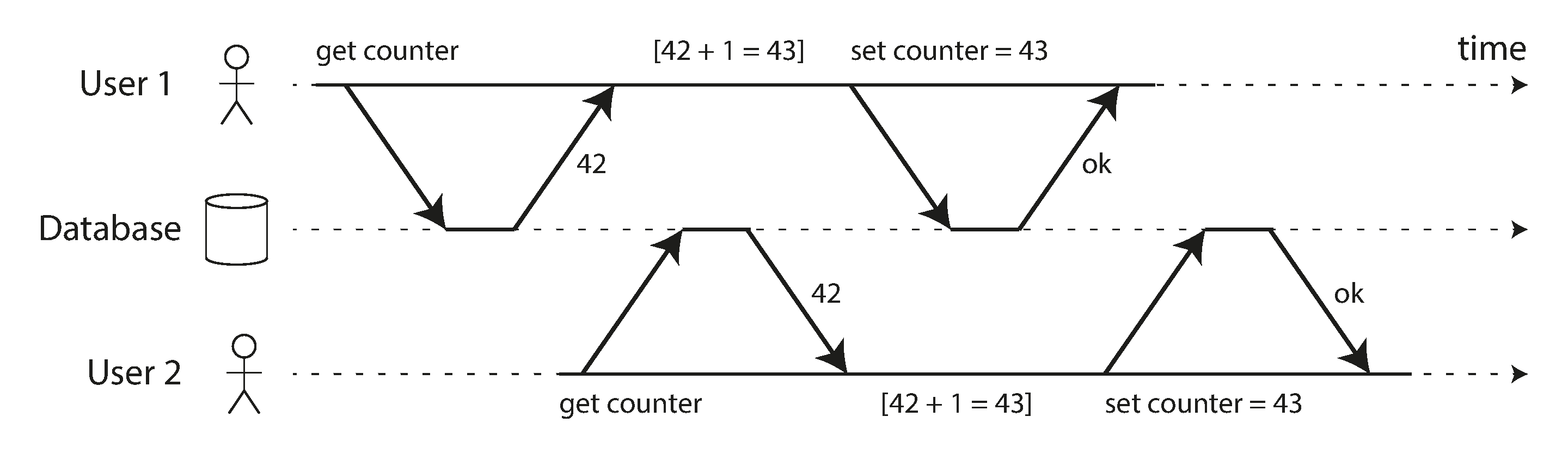
Figure 8-1 A race condition between two clients concurrently incrementing a counter.

Isolation in the sense of ACID means that concurrently executing transactions are isolated from each other: they cannot step on each other’s toes. The classic database textbooks formalize isolation as serializability, which means that each transaction can pretend that it is the only transaction running on the entire database. The database ensures that when the transactions have committed, the result is the same as if they had run serially (one after another), even though in reality they may have run concurrently ¹³.

However, serializability has a performance cost. In practice, many databases use forms of isolation that are weaker than serializability: that is, they allow concurrent transactions to interfere with each other in limited ways. Some popular databases, such as Oracle, don’t even implement it (Oracle has an isolation level called “serializable,” but it actually implements snapshot isolation, which is a weaker guarantee than serializability ¹⁰ ¹⁴). This means that some kinds of race conditions can still occur. We will explore snapshot isolation and other forms of isolation in “Weak Isolation Levels”.

Durability

The purpose of a database system is to provide a safe place where data can be stored without fear of losing it. Durability is the promise that once a transaction has committed successfully, any data it has written will not be forgotten, even if there is a hardware fault or the database crashes.

In a single-node database, durability typically means that the data has been written to nonvolatile storage such as a hard drive or SSD. Regular file writes are usually buffered in memory before being sent to the disk sometime later, which means they would be lost if there is a sudden power failure; many databases therefore use the fsync() system call to ensure the data really has been written to disk. Databases usually also have a write-ahead log or similar (see “Making B-trees reliable”), which allows them to recover in the event that a crash occurs part way through a write.

In a replicated database, durability may mean that the data has been successfully copied to some number of nodes. In order to provide a durability guarantee, a database must wait until these writes or replications are complete before reporting a transaction as successfully committed. However, as discussed in “Reliability and Fault Tolerance”, perfect durability does not exist: if all your hard disks and all your backups are destroyed at the same time, there’s obviously nothing your database can do to save you.

REPLICATION AND DURABILITY

Historically, durability meant writing to an archive tape. Then it was understood as writing to a disk or SSD. More recently, it has been adapted to mean replication. Which implementation is better?

The truth is, nothing is perfect:

If you write to disk and the machine dies, even though your data isn’t lost, it is inaccessible until you either fix the machine or transfer the disk to another machine. Replicated systems can remain available.
A correlated fault—a power outage or a bug that crashes every node on a particular input—can knock out all replicas at once (see “Reliability and Fault Tolerance”), losing any data that is only in memory. Writing to disk is therefore still relevant for replicated databases.
In an asynchronously replicated system, recent writes may be lost when the leader becomes unavailable (see “Handling Node Outages”).
When the power is suddenly cut, SSDs in particular have been shown to sometimes violate the guarantees they are supposed to provide: even fsync isn’t guaranteed to work correctly ¹⁵. Disk firmware can have bugs, just like any other kind of software ¹⁶ ¹⁷, e.g. causing drives to fail after exactly 32,768 hours of operation ¹⁸. And fsync is hard to use; even PostgreSQL used it incorrectly for over 20 years ¹⁹ ²⁰ ²¹.
Subtle interactions between the storage engine and the filesystem implementation can lead to bugs that are hard to track down, and may cause files on disk to be corrupted after a crash ²² ²³. Filesystem errors on one replica can sometimes spread to other replicas as well ²⁴.
Data on disk can gradually become corrupted without this being detected ²⁵. If data has been corrupted for some time, replicas and recent backups may also be corrupted. In this case, you will need to try to restore the data from a historical backup.
One study of SSDs found that between 30% and 80% of drives develop at least one bad block during the first four years of operation, and only some of these can be corrected by the firmware ²⁶. Magnetic hard drives have a lower rate of bad sectors, but a higher rate of complete failure than SSDs.
When a worn-out SSD (that has gone through many write/erase cycles) is disconnected from power, it can start losing data within a timescale of weeks to months, depending on the temperature ²⁷. This is less of a problem for drives with lower wear levels ²⁸.

In practice, there is no one technique that can provide absolute guarantees. There are only various risk-reduction techniques, including writing to disk, replicating to remote machines, and backups—and they can and should be used together. As always, it’s wise to take any theoretical “guarantees” with a healthy grain of salt.

Single-Object and Multi-Object Operations

To recap, in ACID, atomicity and isolation describe what the database should do if a client makes several writes within the same transaction:

Atomicity: If an error occurs halfway through a sequence of writes, the transaction should be aborted, and the writes made up to that point should be discarded. In other words, the database saves you from having to worry about partial failure, by giving an all-or-nothing guarantee.
Isolation: Concurrently running transactions shouldn’t interfere with each other. For example, if one transaction makes several writes, then another transaction should see either all or none of those writes, but not some subset.

These definitions assume that you want to modify several objects (rows, documents, records) at once. Such multi-object transactions are often needed if several pieces of data need to be kept in sync. Figure 8-2 shows an example from an email application. To display the number of unread messages for a user, you could query something like:

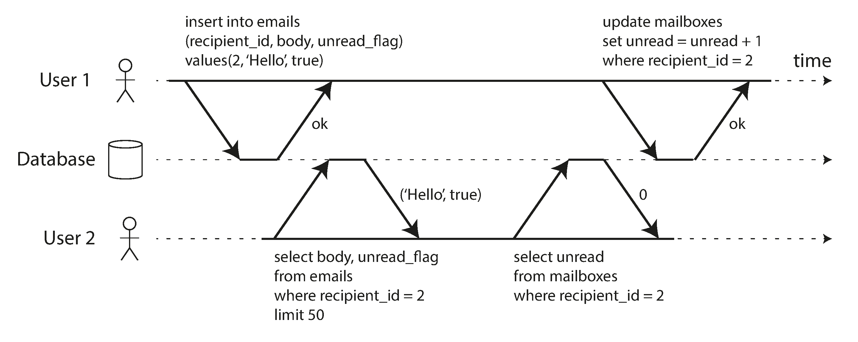
SELECT COUNT(*) FROM emails WHERE recipient_id = 2 AND unread_flag = true

Figure 8-2 Violating isolation: one transaction reads another transaction's uncommitted writes (a "dirty read").

However, you might find this query to be too slow if there are many emails, and decide to store the number of unread messages in a separate field (a kind of denormalization, which we discuss in “Normalization, Denormalization, and Joins”). Now, whenever a new message comes in, you have to increment the unread counter as well, and whenever a message is marked as read, you also have to decrement the unread counter.

In Figure 8-2, user 2 experiences an anomaly: the mailbox listing shows an unread message, but the counter shows zero unread messages because the counter increment has not yet happened. (If an incorrect counter in an email application seems too insignificant, think of a customer account balance instead of an unread counter, and a payment transaction instead of an email.) Isolation would have prevented this issue by ensuring that user 2 sees either both the inserted email and the updated counter, or neither, but not an inconsistent halfway point.

Figure 8-3 illustrates the need for atomicity: if an error occurs somewhere over the course of the transaction, the contents of the mailbox and the unread counter might become out of sync. In an atomic transaction, if the update to the counter fails, the transaction is aborted and the inserted email is rolled back.

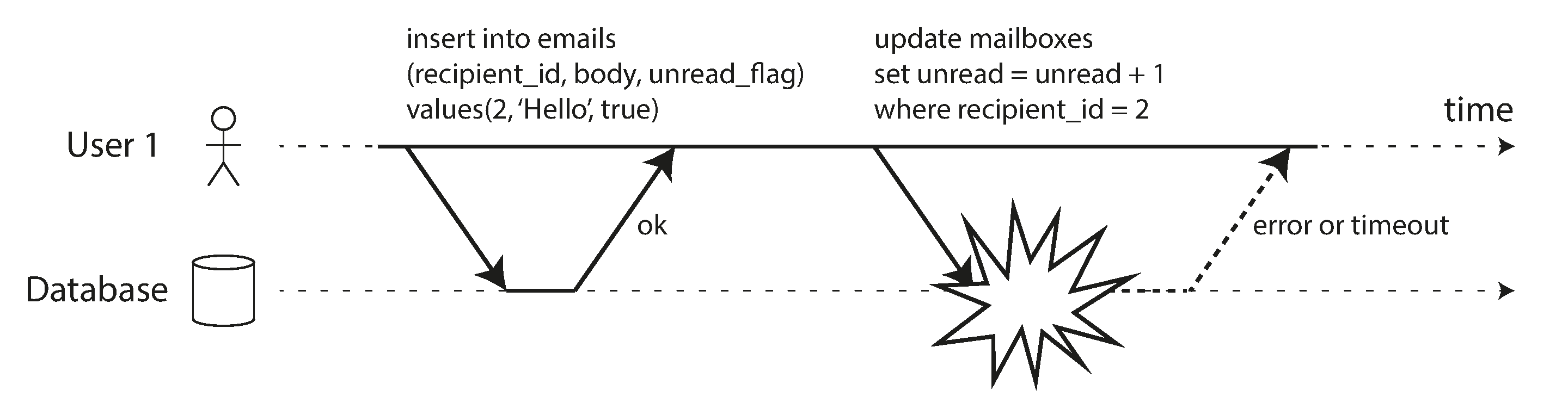
Figure 8-3 Atomicity ensures that if an error occurs any prior writes from that transaction are undone, to avoid an inconsistent state.

Multi-object transactions require some way of determining which read and write operations belong to the same transaction. In relational databases, that is typically done based on the client’s TCP connection to the database server: on any particular connection, everything between a BEGIN TRANSACTION and a COMMIT statement is considered to be part of the same transaction. If the TCP connection is interrupted, the transaction must be aborted.

On the other hand, many nonrelational databases don’t have such a way of grouping operations together. Even if there is a multi-object API (for example, a key-value store may have a multi-put operation that updates several keys in one operation), that doesn’t necessarily mean it has transaction semantics: the command may succeed for some keys and fail for others, leaving the database in a partially updated state.

Single-object writes

Atomicity and isolation also apply when a single object is being changed. For example, imagine you are writing a 20 KB JSON document to a database:

If the network connection is interrupted after the first 10 KB have been sent, does the database store that unparseable 10 KB fragment of JSON?
If the power fails while the database is in the middle of overwriting the previous value on disk, do you end up with the old and new values spliced together?
If another client reads that document while the write is in progress, will it see a partially updated value?

Those issues would be incredibly confusing, so storage engines almost universally aim to provide atomicity and isolation on the level of a single object (such as a key-value pair) on one node. Atomicity can be implemented using a log for crash recovery (see “Making B-trees reliable”), and isolation can be implemented using a lock on each object (allowing only one thread to access an object at any one time).

Some databases also provide more complex atomic operations, such as an increment operation, which removes the need for a read-modify-write cycle like that in Figure 8-1. Similarly popular is a conditional write operation, which allows a write to happen only if the value has not been concurrently changed by someone else (see “Conditional writes (compare-and-set)”), similarly to a compare-and-set or compare-and-swap (CAS) operation in shared-memory concurrency.

Note

Strictly speaking, the term atomic increment uses the word atomic in the sense of multi-threaded programming. In the context of ACID, it should actually be called an isolated or serializable increment, but that’s not the usual term.

These single-object operations are useful, as they can prevent lost updates when several clients try to write to the same object concurrently (see “Preventing Lost Updates”). However, they are not transactions in the usual sense of the word. For example, the “lightweight transactions” feature of Cassandra and ScyllaDB, and Aerospike’s “strong consistency” mode offer linearizable (see “Linearizability”) reads and conditional writes on a single object, but no guarantees across multiple objects.

The need for multi-object transactions

Do we need multi-object transactions at all? Would it be possible to implement any application with only a key-value data model and single-object operations?

There are some use cases in which single-object inserts, updates, and deletes are sufficient. However, in many other cases writes to several different objects need to be coordinated:

In a relational data model, a row in one table often has a foreign key reference to a row in another table. Similarly, in a graph-like data model, a vertex has edges to other vertices. Multi-object transactions allow you to ensure that these references remain valid: when inserting several records that refer to one another, the foreign keys have to be correct and up to date, or the data becomes nonsensical.
In a document data model, the fields that need to be updated together are often within the same document, which is treated as a single object—no multi-object transactions are needed when updating a single document. However, document databases lacking join functionality also encourage denormalization (see “When to Use Which Model”). When denormalized information needs to be updated, like in the example of Figure 8-2, you need to update several documents in one go. Transactions are very useful in this situation to prevent denormalized data from going out of sync.
In databases with secondary indexes (almost everything except pure key-value stores), the indexes also need to be updated every time you change a value. These indexes are different database objects from a transaction point of view: for example, without transaction isolation, it’s possible for a record to appear in one index but not another, because the update to the second index hasn’t happened yet (see “Sharding and Secondary Indexes”).

Such applications can still be implemented without transactions. However, error handling becomes much more complicated without atomicity, and the lack of isolation can cause concurrency problems. We will discuss those in “Weak Isolation Levels”, and explore alternative approaches in “Derived data versus distributed transactions”.

Handling errors and aborts

A key feature of a transaction is that it can be aborted and safely retried if an error occurred. ACID databases are based on this philosophy: if the database is in danger of violating its guarantee of atomicity, isolation, or durability, it would rather abandon the transaction entirely than allow it to remain half-finished.

Not all systems follow that philosophy, though. In particular, datastores with leaderless replication (see “Leaderless Replication”) work much more on a “best effort” basis, which could be summarized as “the database will do as much as it can, and if it runs into an error, it won’t undo something it has already done”—so it’s the application’s responsibility to recover from errors.

Errors will inevitably happen, but many software developers prefer to think only about the happy path rather than the intricacies of error handling. For example, popular object-relational mapping (ORM) frameworks such as Rails’s ActiveRecord and Django don’t retry aborted transactions—the error usually results in an exception bubbling up the stack, so any user input is thrown away and the user gets an error message. This is a shame, because the whole point of aborts is to enable safe retries.

Although retrying an aborted transaction is a simple and effective error handling mechanism, it isn’t perfect:

If the transaction actually succeeded, but the network was interrupted while the server tried to acknowledge the successful commit to the client (so it timed out from the client’s point of view), then retrying the transaction causes it to be performed twice—unless you have an additional application-level deduplication mechanism in place.
If the error is due to overload or high contention between concurrent transactions, retrying the transaction will make the problem worse, not better. To avoid such feedback cycles, you can limit the number of retries, use exponential backoff, and handle overload-related errors differently from other errors (see “When an overloaded system won’t recover”).
It is only worth retrying after transient errors (for example due to deadlock, isolation violation, temporary network interruptions, and failover); after a permanent error (e.g., constraint violation) a retry would be pointless.
If the transaction also has side effects outside of the database, those side effects may happen even if the transaction is aborted. For example, if you’re sending an email, you wouldn’t want to send the email again every time you retry the transaction. If you want to make sure that several different systems either commit or abort together, two-phase commit can help (we will discuss this in “Two-Phase Commit (2PC)”).
If the client process crashes while retrying, any data it was trying to write to the database is lost.

Weak Isolation Levels

If two transactions don’t access the same data, or if both are read-only, they can safely be run in parallel, because neither depends on the other. Concurrency issues (race conditions) only come into play when one transaction reads data that is concurrently modified by another transaction, or when the two transactions try to modify the same data.

Concurrency bugs are hard to find by testing, because such bugs are only triggered when you get unlucky with the timing. Such timing issues might occur very rarely, and are usually difficult to reproduce. Concurrency is also very difficult to reason about, especially in a large application where you don’t necessarily know which other pieces of code are accessing the database. Application development is difficult enough if you just have one user at a time; having many concurrent users makes it much harder still, because any piece of data could unexpectedly change at any time.

For that reason, databases have long tried to hide concurrency issues from application developers by providing transaction isolation. In theory, isolation should make your life easier by letting you pretend that no concurrency is happening: serializable isolation means that the database guarantees that transactions have the same effect as if they ran serially (i.e., one at a time, without any concurrency).

In practice, isolation is unfortunately not that simple. Serializable isolation has a performance cost, and many databases don’t want to pay that price ¹⁰. It’s therefore common for systems to use weaker levels of isolation, which protect against some concurrency issues, but not all. Those levels of isolation are much harder to understand, and they can lead to subtle bugs, but they are nevertheless used in practice ²⁹.

Concurrency bugs caused by weak transaction isolation are not just a theoretical problem. They have caused substantial loss of money ³⁰ ³¹ ³², led to investigation by financial auditors ³³, and caused customer data to be corrupted ³⁴. A popular comment on revelations of such problems is “Use an ACID database if you’re handling financial data!”—but that misses the point. Even many popular relational database systems (which are usually considered “ACID”) use weak isolation, so they wouldn’t necessarily have prevented these bugs from occurring.

Note

Incidentally, much of the banking system relies on text files that are exchanged via secure FTP ³⁵. In this context, having an audit trail and some human-level fraud prevention measures is actually more important than ACID properties.

Those examples also highlight an important point: even if concurrency issues are rare in normal operation, you have to consider the possibility that an attacker deliberately sends a burst of highly concurrent requests to your API in an attempt to deliberately exploit concurrency bugs ³⁰. Therefore, in order to build applications that are reliable and secure, you have to ensure that such bugs are systematically prevented.

In this section we will look at several weak (nonserializable) isolation levels that are used in practice, and discuss in detail what kinds of race conditions can and cannot occur, so that you can decide what level is appropriate to your application. Once we’ve done that, we will discuss serializability in detail (see “Serializability”). Our discussion of isolation levels will be informal, using examples. If you want rigorous definitions and analyses of their properties, you can find them in the academic literature ³⁶ ³⁷ ³⁸ ³⁹.

Read Committed

The most basic level of transaction isolation is read committed. It makes two guarantees:

When reading from the database, you will only see data that has been committed (no dirty reads).
When writing to the database, you will only overwrite data that has been committed (no dirty writes).

Some databases support an even weaker isolation level called read uncommitted. It prevents dirty writes, but does not prevent dirty reads. Let’s discuss these two guarantees in more detail.

No dirty reads

Imagine a transaction has written some data to the database, but the transaction has not yet committed or aborted. Can another transaction see that uncommitted data? If yes, that is called a dirty read ³.

Transactions running at the read committed isolation level must prevent dirty reads. This means that any writes by a transaction only become visible to others when that transaction commits (and then all of its writes become visible at once). This is illustrated in Figure 8-4, where user 1 has set x = 3, but user 2’s get x still returns the old value, 2, while user 1 has not yet committed.

Figure 8-4 No dirty reads: user 2 sees the new value for x only after user 1's transaction has committed.

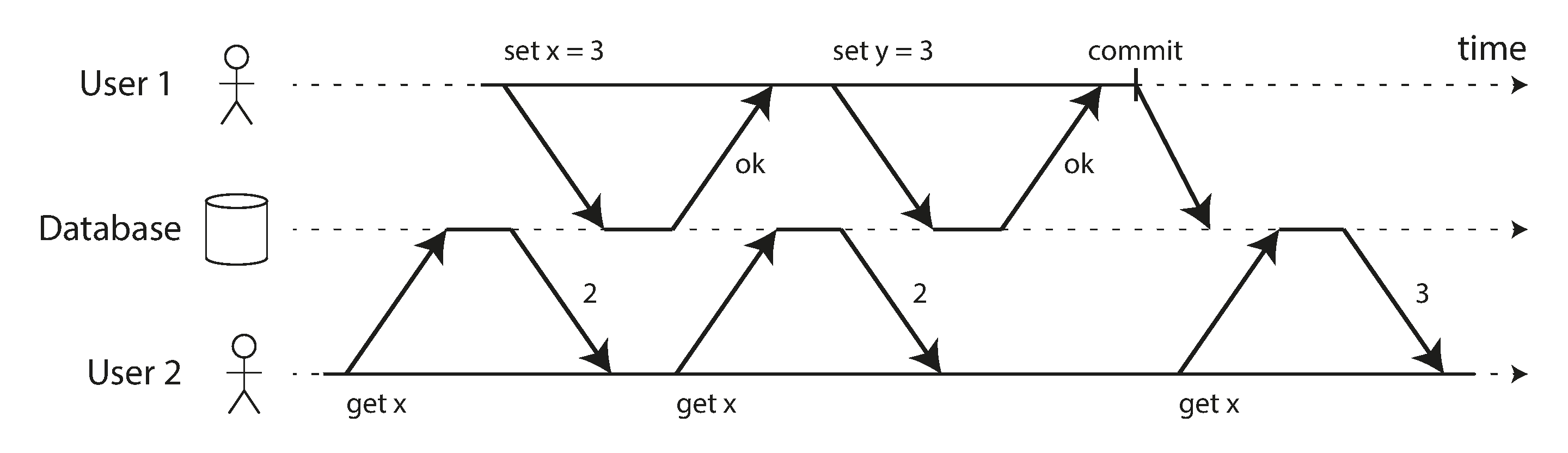
There are a few reasons why it’s useful to prevent dirty reads:

If a transaction needs to update several rows, a dirty read means that another transaction may see some of the updates but not others. For example, in Figure 8-2, the user sees the new unread email but not the updated counter. This is a dirty read of the email. Seeing the database in a partially updated state is confusing to users and may cause other transactions to take incorrect decisions.
If a transaction aborts, any writes it has made need to be rolled back (like in Figure 8-3). If the database allows dirty reads, that means a transaction may see data that is later rolled back—i.e., which is never actually committed to the database. Any transaction that read uncommitted data would also need to be aborted, leading to a problem called cascading aborts.

No dirty writes

What happens if two transactions concurrently try to update the same row in a database? We don’t know in which order the writes will happen, but we normally assume that the later write overwrites the earlier write.

However, what happens if the earlier write is part of a transaction that has not yet committed, so the later write overwrites an uncommitted value? This is called a dirty write ³⁶. Transactions running at the read committed isolation level must prevent dirty writes, usually by delaying the second write until the first write’s transaction has committed or aborted.

By preventing dirty writes, this isolation level avoids some kinds of concurrency problems:

If transactions update multiple rows, dirty writes can lead to a bad outcome. For example, consider Figure 8-5, which illustrates a used car sales website on which two people, Aaliyah and Bryce, are simultaneously trying to buy the same car. Buying a car requires two database writes: the listing on the website needs to be updated to reflect the buyer, and the sales invoice needs to be sent to the buyer. In the case of Figure 8-5, the sale is awarded to Bryce (because he performs the winning update to the listings table), but the invoice is sent to Aaliyah (because she performs the winning update to the invoices table). Read committed prevents such mishaps.
However, read committed does not prevent the race condition between two counter increments in Figure 8-1. In this case, the second write happens after the first transaction has committed, so it’s not a dirty write. It’s still incorrect, but for a different reason—in “Preventing Lost Updates” we will discuss how to make such counter increments safe.

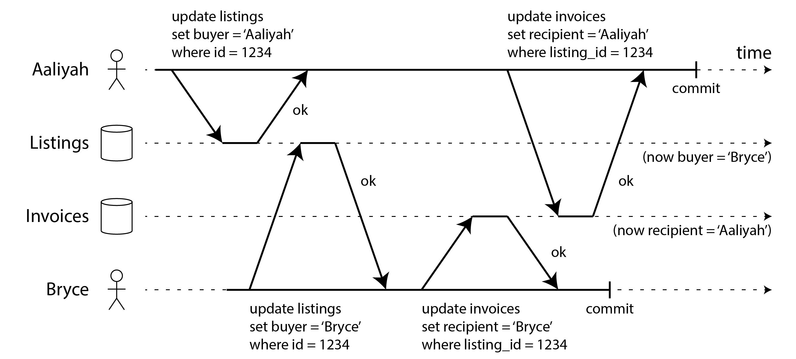
Figure 8-5 With dirty writes, conflicting writes from different transactions can be mixed up.

Implementing read committed

Read committed is a very popular isolation level. It is the default setting in Oracle Database, PostgreSQL, SQL Server, and many other databases ¹⁰.

Most commonly, databases prevent dirty writes by using row-level locks: when a transaction wants to modify a particular row (or document or some other object), it must first acquire a lock on that row. It must then hold that lock until the transaction is committed or aborted. Only one transaction can hold the lock for any given row; if another transaction wants to write to the same row, it must wait until the first transaction is committed or aborted before it can acquire the lock and continue. This locking is done automatically by databases in read committed mode (or stronger isolation levels).

How do we prevent dirty reads? One option would be to use the same lock, and to require any transaction that wants to read a row to briefly acquire the lock and then release it again immediately after reading. This would ensure that a read couldn’t happen while a row has a dirty, uncommitted value (because during that time the lock would be held by the transaction that has made the write).

However, the approach of requiring read locks does not work well in practice, because one long-running write transaction can force many other transactions to wait until the long-running transaction has completed, even if the other transactions only read and do not write anything to the database. This harms the response time of read-only transactions and is bad for operability: a slowdown in one part of an application can have a knock-on effect in a completely different part of the application, due to waiting for locks.

Nevertheless, locks are used to prevent dirty reads in some databases, such as IBM Db2 and Microsoft SQL Server in the read_committed_snapshot=off setting ²⁹.

A more commonly used approach to preventing dirty reads is the one illustrated in Figure 8-4: for every row that is written, the database remembers both the old committed value and the new value set by the transaction that currently holds the write lock. While the transaction is ongoing, any other transactions that read the row are simply given the old value. Only when the new value is committed do transactions switch over to reading the new value (see “Multi-version concurrency control (MVCC)” for more detail).

Snapshot Isolation and Repeatable Read

If you look superficially at read committed isolation, you could be forgiven for thinking that it does everything that a transaction needs to do: it allows aborts (required for atomicity), it prevents reading the incomplete results of transactions, and it prevents concurrent writes from getting intermingled. Indeed, those are useful features, and much stronger guarantees than you can get from a system that has no transactions.

However, there are still plenty of ways in which you can have concurrency bugs when using this isolation level. For example, Figure 8-6 illustrates a problem that can occur with read committed.

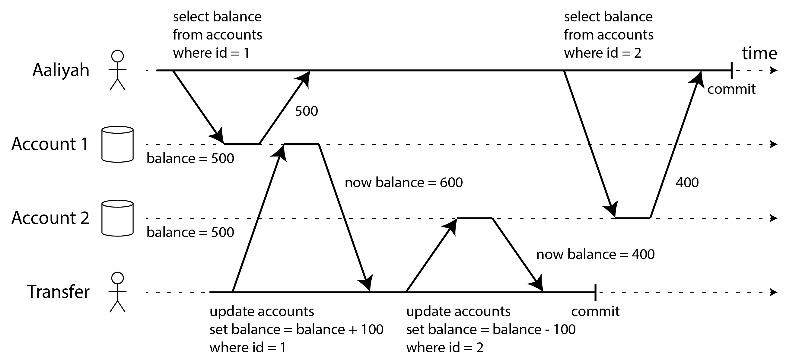
Figure 8-6 Read skew: Aaliyah observes the database in an inconsistent state.

Say Aaliyah has $1,000 of savings at a bank, split across two accounts with $500 each. Now a transaction transfers $100 from one of her accounts to the other. If she is unlucky enough to look at her list of account balances in the same moment as that transaction is being processed, she may see one account balance at a time before the incoming payment has arrived (with a balance of $500), and the other account after the outgoing transfer has been made (the new balance being $400). To Aaliyah it now appears as though she only has a total of $900 in her accounts—it seems that $100 has vanished into thin air.

This anomaly is called read skew, and it is an example of a nonrepeatable read: if Aaliyah were to read the balance of account 1 again at the end of the transaction, she would see a different value ($600) than she saw in her previous query. Read skew is considered acceptable under read committed isolation: the account balances that Aaliyah saw were indeed committed at the time when she read them.

Note

The term skew is unfortunately overloaded: we previously used it in the sense of an unbalanced workload with hot spots (see “Skewed Workloads and Relieving Hot Spots”), whereas here it means timing anomaly.

In Aaliyah’s case, this is not a lasting problem, because she will most likely see consistent account balances if she reloads the online banking website a few seconds later. However, some situations cannot tolerate such temporary inconsistency:

Backups: Taking a backup requires making a copy of the entire database, which may take hours on a large database. During the time that the backup process is running, writes will continue to be made to the database. Thus, you could end up with some parts of the backup containing an older version of the data, and other parts containing a newer version. If you need to restore from such a backup, the inconsistencies (such as disappearing money) become permanent.
Analytic queries and integrity checks: Sometimes, you may want to run a query that scans over large parts of the database. Such queries are common in analytics (see “Analytical versus Operational Systems”), or may be part of a periodic integrity check that everything is in order (monitoring for data corruption). These queries are likely to return nonsensical results if they observe parts of the database at different points in time.

Snapshot isolation ³⁶ is the most common solution to this problem. The idea is that each transaction reads from a consistent snapshot of the database—that is, the transaction sees all the data that was committed in the database at the start of the transaction. Even if the data is subsequently changed by another transaction, each transaction sees only the old data from that particular point in time.

Snapshot isolation is a boon for long-running, read-only queries such as backups and analytics. It is very hard to reason about the meaning of a query if the data on which it operates is changing at the same time as the query is executing. When a transaction can see a consistent snapshot of the database, frozen at a particular point in time, it is much easier to understand.

Snapshot isolation is a popular feature: variants of it are supported by PostgreSQL, MySQL with the InnoDB storage engine, Oracle, SQL Server, and others, although the detailed behavior varies from one system to the next ²⁹ ⁴⁰ ⁴¹. Some databases, such as Oracle, TiDB, and Aurora DSQL, even choose snapshot isolation as their highest isolation level.

Multi-version concurrency control (MVCC)

Like read committed isolation, implementations of snapshot isolation typically use write locks to prevent dirty writes (see “Implementing read committed”), which means that a transaction that makes a write can block the progress of another transaction that writes to the same row. However, reads do not require any locks. From a performance point of view, a key principle of snapshot isolation is readers never block writers, and writers never block readers. This allows a database to handle long-running read queries on a consistent snapshot at the same time as processing writes normally, without any lock contention between the two.

To implement snapshot isolation, databases use a generalization of the mechanism we saw for preventing dirty reads in Figure 8-4. Instead of two versions of each row (the committed version and the overwritten-but-not-yet-committed version), the database must potentially keep several different committed versions of a row, because various in-progress transactions may need to see the state of the database at different points in time. Because it maintains several versions of a row side by side, this technique is known as multi-version concurrency control (MVCC).

Figure 8-7 illustrates how MVCC-based snapshot isolation is implemented in PostgreSQL ⁴⁰ ⁴² ⁴³ (other implementations are similar). When a transaction is started, it is given a unique, always-increasing transaction ID (txid). Whenever a transaction writes anything to the database, the data it writes is tagged with the transaction ID of the writer. (To be precise, transaction IDs in PostgreSQL are 32-bit integers, so they overflow after approximately 4 billion transactions. The vacuum process performs cleanup to ensure that overflow does not affect the data.)

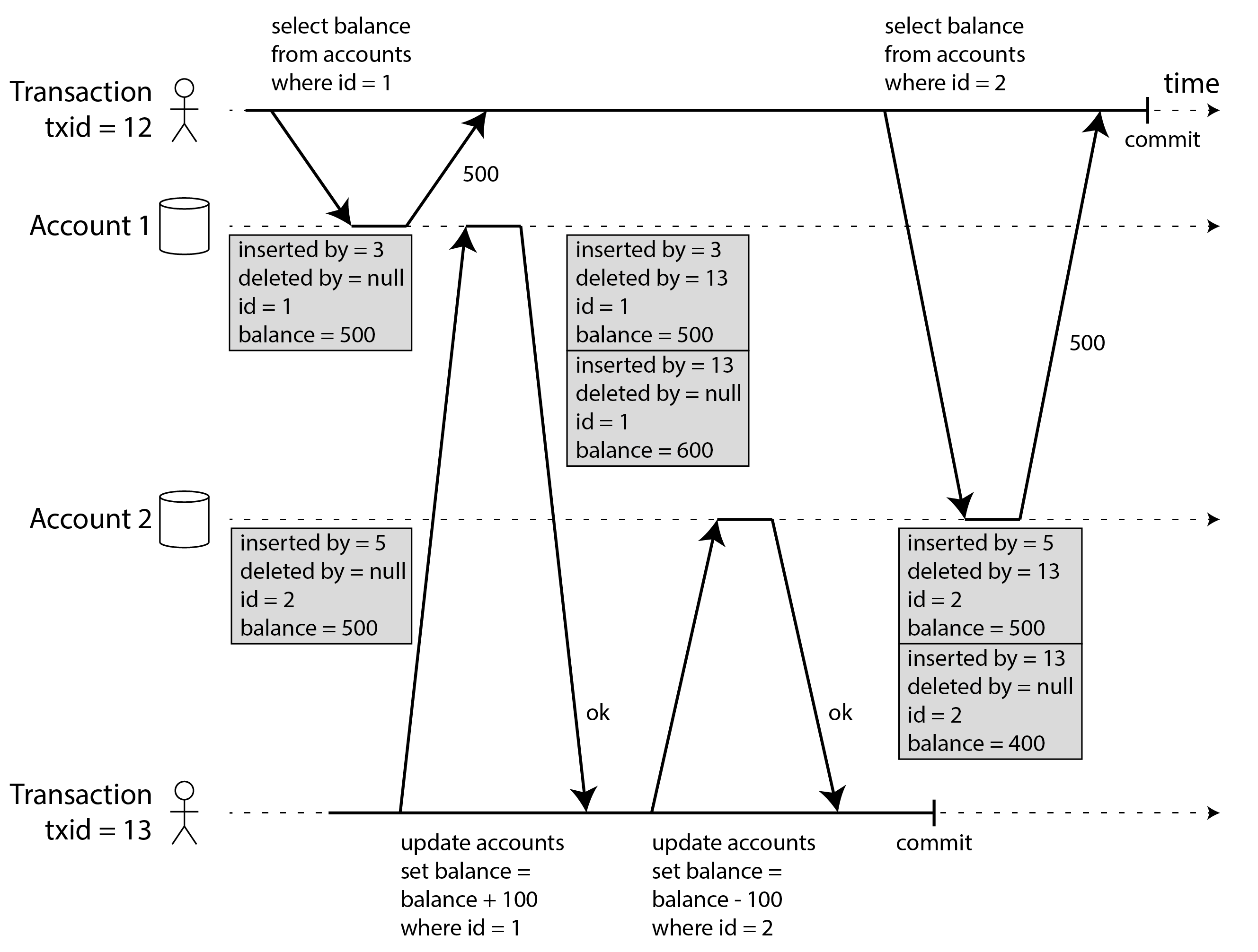
Figure 8-7 Implementing snapshot isolation using multi-version concurrency control.

Each row in a table has a inserted_by field, containing the ID of the transaction that inserted this row into the table. Moreover, each row has a deleted_by field, which is initially empty. If a transaction deletes a row, the row isn’t actually removed from the database, but it is marked for deletion by setting the deleted_by field to the ID of the transaction that requested the deletion. At some later time, when it is certain that no transaction can any longer access the deleted data, a garbage collection process in the database removes any rows marked for deletion and frees their space.

An update is internally translated into a delete and a insert ⁴⁴. For example, in Figure 8-7, transaction 13 deducts $100 from account 2, changing the balance from $500 to $400. The accounts table now actually contains two rows for account 2: a row with a balance of $500 which was marked as deleted by transaction 13, and a row with a balance of $400 which was inserted by transaction 13.

All of the versions of a row are stored within the same database heap (see “Storing values within the index”), regardless of whether the transactions that wrote them have committed or not. The versions of the same row form a linked list, going either from newest version to oldest version or the other way round, so that queries can internally iterate over all versions of a row ⁴⁵ ⁴⁶.

Visibility rules for observing a consistent snapshot

When a transaction reads from the database, transaction IDs are used to decide which row versions it can see and which are invisible. By carefully defining visibility rules, the database can present a consistent snapshot of the database to the application. This works roughly as follows ⁴³:

At the start of each transaction, the database makes a list of all the other transactions that are in progress (not yet committed or aborted) at that time. Any writes that those transactions have made are ignored, even if the transactions subsequently commit. This ensures that we see a consistent snapshot that is not affected by another transaction committing.
Any writes made by transactions with a later transaction ID (i.e., which started after the current transaction started, and which are therefore not included in the list of in-progress transactions) are ignored, regardless of whether those transactions have committed.
Any writes made by aborted transactions are ignored, regardless of when that abort happened. This has the advantage that when a transaction aborts, we don’t need to immediately remove the rows it wrote from storage, since the visibility rule filters them out. The garbage collection process can remove them later.
All other writes are visible to the application’s queries.

These rules apply to both insertion and deletion of rows. In Figure 8-7, when transaction 12 reads from account 2, it sees a balance of $500 because the deletion of the $500 balance was made by transaction 13 (according to rule 2, transaction 12 cannot see a deletion made by transaction 13), and the insertion of the $400 balance is not yet visible (by the same rule).

Put another way, a row is visible if both of the following conditions are true:

At the time when the reader’s transaction started, the transaction that inserted the row had already committed.
The row is not marked for deletion, or if it is, the transaction that requested deletion had not yet committed at the time when the reader’s transaction started.

A long-running transaction may continue using a snapshot for a long time, continuing to read values that (from other transactions’ point of view) have long been overwritten or deleted. By never updating values in place but instead inserting a new version every time a value is changed, the database can provide a consistent snapshot while incurring only a small overhead.

Indexes and snapshot isolation

How do indexes work in a multi-version database? The most common approach is that each index entry points at one of the versions of a row that matches the entry (either the oldest or the newest version). Each row version may contain a reference to the next-oldest or next-newest version. A query that uses the index must then iterate over the rows to find one that is visible, and where the value matches what the query is looking for. When garbage collection removes old row versions that are no longer visible to any transaction, the corresponding index entries can also be removed.

Many implementation details affect the performance of multi-version concurrency control ⁴⁵ ⁴⁶. For example, PostgreSQL has optimizations for avoiding index updates if different versions of the same row can fit on the same page ⁴⁰. Some other databases avoid storing full copies of modified rows, and only store differences between versions to save space.

Another approach is used in CouchDB, Datomic, and LMDB. Although they also use B-trees (see “B-Trees”), they use an immutable (copy-on-write) variant that does not overwrite pages of the tree when they are updated, but instead creates a new copy of each modified page. Parent pages, up to the root of the tree, are copied and updated to point to the new versions of their child pages. Any pages that are not affected by a write do not need to be copied, and can be shared with the new tree ⁴⁷.

With immutable B-trees, every write transaction (or batch of transactions) creates a new B-tree root, and a particular root is a consistent snapshot of the database at the point in time when it was created. There is no need to filter out rows based on transaction IDs because subsequent writes cannot modify an existing B-tree; they can only create new tree roots. This approach also requires a background process for compaction and garbage collection.

Snapshot isolation, repeatable read, and naming confusion

MVCC is a commonly used implementation technique for databases, and often it is used to implement snapshot isolation. However, different databases sometimes use different terms to refer to the same thing: for example, snapshot isolation is called “repeatable read” in PostgreSQL, and “serializable” in Oracle ²⁹. Sometimes different systems use the same term to mean different things: for example, while in PostgreSQL “repeatable read” means snapshot isolation, in MySQL it means an implementation of MVCC with weaker consistency than snapshot isolation ⁴¹.

The reason for this naming confusion is that the SQL standard doesn’t have the concept of snapshot isolation, because the standard is based on System R’s 1975 definition of isolation levels ³ and snapshot isolation hadn’t yet been invented then. Instead, it defines repeatable read, which looks superficially similar to snapshot isolation. PostgreSQL calls its snapshot isolation level “repeatable read” because it meets the requirements of the standard, and so they can claim standards compliance.

Unfortunately, the SQL standard’s definition of isolation levels is flawed—it is ambiguous, imprecise, and not as implementation-independent as a standard should be ³⁶. Even though several databases implement repeatable read, there are big differences in the guarantees they actually provide, despite being ostensibly standardized ²⁹. There has been a formal definition of repeatable read in the research literature ³⁷ ³⁸, but most implementations don’t satisfy that formal definition. And to top it off, IBM Db2 uses “repeatable read” to refer to serializability ¹⁰.

As a result, nobody really knows what repeatable read means.

Preventing Lost Updates

The read committed and snapshot isolation levels we’ve discussed so far have been primarily about the guarantees of what a read-only transaction can see in the presence of concurrent writes. We have mostly ignored the issue of two transactions writing concurrently—we have only discussed dirty writes (see “No dirty writes”), one particular type of write-write conflict that can occur.

There are several other interesting kinds of conflicts that can occur between concurrently writing transactions. The best known of these is the lost update problem, illustrated in Figure 8-1 with the example of two concurrent counter increments.

The lost update problem can occur if an application reads some value from the database, modifies it, and writes back the modified value (a read-modify-write cycle). If two transactions do this concurrently, one of the modifications can be lost, because the second write does not include the first modification. (We sometimes say that the later write clobbers the earlier write.) This pattern occurs in various different scenarios:

Incrementing a counter or updating an account balance (requires reading the current value, calculating the new value, and writing back the updated value)
Making a local change to a complex value, e.g., adding an element to a list within a JSON document (requires parsing the document, making the change, and writing back the modified document)
Two users editing a wiki page at the same time, where each user saves their changes by sending the entire page contents to the server, overwriting whatever is currently in the database

Because this is such a common problem, a variety of solutions have been developed ⁴⁸.

Atomic write operations

Many databases provide atomic update operations, which remove the need to implement read-modify-write cycles in application code. They are usually the best solution if your code can be expressed in terms of those operations. For example, the following instruction is concurrency-safe in most relational databases:

UPDATE counters SET value = value + 1 WHERE key = 'foo';

Similarly, document databases such as MongoDB provide atomic operations for making local modifications to a part of a JSON document, and Redis provides atomic operations for modifying data structures such as priority queues. Not all writes can easily be expressed in terms of atomic operations—for example, updates to a wiki page involve arbitrary text editing, which can be handled using algorithms discussed in “CRDTs and Operational Transformation”—but in situations where atomic operations can be used, they are usually the best choice.

Atomic operations are usually implemented by taking an exclusive lock on the object when it is read so that no other transaction can read it until the update has been applied. Another option is to simply force all atomic operations to be executed on a single thread.

Unfortunately, object-relational mapping (ORM) frameworks make it easy to accidentally write code that performs unsafe read-modify-write cycles instead of using atomic operations provided by the database ⁴⁹ ⁵⁰ ⁵¹. This can be a source of subtle bugs that are difficult to find by testing.

Explicit locking

Another option for preventing lost updates, if the database’s built-in atomic operations don’t provide the necessary functionality, is for the application to explicitly lock objects that are going to be updated. Then the application can perform a read-modify-write cycle, and if any other transaction tries to concurrently update or lock the same object, it is forced to wait until the first read-modify-write cycle has completed.

For example, consider a multiplayer game in which several players can move the same figure concurrently. In this case, an atomic operation may not be sufficient, because the application also needs to ensure that a player’s move abides by the rules of the game, which involves some logic that you cannot sensibly implement as a database query. Instead, you may use a lock to prevent two players from concurrently moving the same piece, as illustrated in Example 8-1.

Example 8-1. Explicitly locking rows to prevent lost updates

BEGIN TRANSACTION;

SELECT * FROM figures
    WHERE name = 'robot' AND game_id = 222
    FOR UPDATE; ❶

-- Check whether move is valid, then update the position
-- of the piece that was returned by the previous SELECT.
UPDATE figures SET position = 'c4' WHERE id = 1234;

COMMIT;

❶: The FOR UPDATE clause indicates that the database should take a lock on all rows returned by this query.

This works, but to get it right, you need to carefully think about your application logic. It’s easy to forget to add a necessary lock somewhere in the code, and thus introduce a race condition.

Moreover, if you lock multiple objects there is a risk of deadlock, where two or more transactions are waiting for each other to release their locks. Many databases automatically detect deadlocks, and abort one of the involved transactions so that the system can make progress. You can handle this situation at the application level by retrying the aborted transaction.

Automatically detecting lost updates

Atomic operations and locks are ways of preventing lost updates by forcing the read-modify-write cycles to happen sequentially. An alternative is to allow them to execute in parallel and, if the transaction manager detects a lost update, abort the transaction and force it to retry its read-modify-write cycle.

An advantage of this approach is that databases can perform this check efficiently in conjunction with snapshot isolation. Indeed, PostgreSQL’s repeatable read, Oracle’s serializable, and SQL Server’s snapshot isolation levels automatically detect when a lost update has occurred and abort the offending transaction. However, MySQL/InnoDB’s repeatable read does not detect lost updates ²⁹ ⁴¹. Some authors ³⁶ ³⁸ argue that a database must prevent lost updates in order to qualify as providing snapshot isolation, so MySQL does not provide snapshot isolation under this definition.

Lost update detection is a great feature, because it doesn’t require application code to use any special database features—you may forget to use a lock or an atomic operation and thus introduce a bug, but lost update detection happens automatically and is thus less error-prone. However, you also have to retry aborted transactions at the application level.

Conditional writes (compare-and-set)

In databases that don’t provide transactions, you sometimes find a conditional write operation that can prevent lost updates by allowing an update to happen only if the value has not changed since you last read it (previously mentioned in “Single-object writes”). If the current value does not match what you previously read, the update has no effect, and the read-modify-write cycle must be retried. It is the database equivalent of an atomic compare-and-set or compare-and-swap (CAS) instruction that is supported by many CPUs.

For example, to prevent two users concurrently updating the same wiki page, you might try something like this, expecting the update to occur only if the content of the page hasn’t changed since the user started editing it:

-- This may or may not be safe, depending on the database implementation
UPDATE wiki_pages SET content = 'new content'
    WHERE id = 1234 AND content = 'old content';

If the content has changed and no longer matches 'old content', this update will have no effect, so you need to check whether the update took effect and retry if necessary. Instead of comparing the full content, you could also use a version number column that you increment on every update, and apply the update only if the current version number hasn’t changed. This approach is sometimes called optimistic locking ⁵².

Note that if another transaction has concurrently modified content, the new content may not be visible under the MVCC visibility rules (see “Visibility rules for observing a consistent snapshot”). Many implementations of MVCC have an exception to the visibility rules for this scenario, where values written by other transactions are visible to the evaluation of the WHERE clause of UPDATE and DELETE queries, even though those writes are not otherwise visible in the snapshot.

Conflict resolution and replication

In replicated databases (see Chapter 6), preventing lost updates takes on another dimension: since they have copies of the data on multiple nodes, and the data can potentially be modified concurrently on different nodes, some additional steps need to be taken to prevent lost updates.

Locks and conditional write operations assume that there is a single up-to-date copy of the data. However, databases with multi-leader or leaderless replication usually allow several writes to happen concurrently and replicate them asynchronously, so they cannot guarantee that there is a single up-to-date copy of the data. Thus, techniques based on locks or conditional writes do not apply in this context. (We will revisit this issue in more detail in “Linearizability”.)

Instead, as discussed in “Dealing with Conflicting Writes”, a common approach in such replicated databases is to allow concurrent writes to create several conflicting versions of a value (also known as siblings), and to use application code or special data structures to resolve and merge these versions after the fact.

Merging conflicting values can prevent lost updates if the updates are commutative (i.e., you can apply them in a different order on different replicas, and still get the same result). For example, incrementing a counter or adding an element to a set are commutative operations. That is the idea behind CRDTs, which we encountered in “CRDTs and Operational Transformation”. However, some operations such as conditional writes cannot be made commutative.

On the other hand, the last write wins (LWW) conflict resolution method is prone to lost updates, as discussed in “Last write wins (discarding concurrent writes)”. Unfortunately, LWW is the default in many replicated databases.

Write Skew and Phantoms

In the previous sections we saw dirty writes and lost updates, two kinds of race conditions that can occur when different transactions concurrently try to write to the same objects. In order to avoid data corruption, those race conditions need to be prevented—either automatically by the database, or by manual safeguards such as using locks or atomic write operations.

However, that is not the end of the list of potential race conditions that can occur between concurrent writes. In this section we will see some subtler examples of conflicts.

To begin, imagine this example: you are writing an application for doctors to manage their on-call shifts at a hospital. The hospital usually tries to have several doctors on call at any one time, but it absolutely must have at least one doctor on call. Doctors can give up their shifts (e.g., if they are sick themselves), provided that at least one colleague remains on call in that shift ⁵³ ⁵⁴.

Now imagine that Aaliyah and Bryce are the two on-call doctors for a particular shift. Both are feeling unwell, so they both decide to request leave. Unfortunately, they happen to click the button to go off call at approximately the same time. What happens next is illustrated in Figure 8-8.

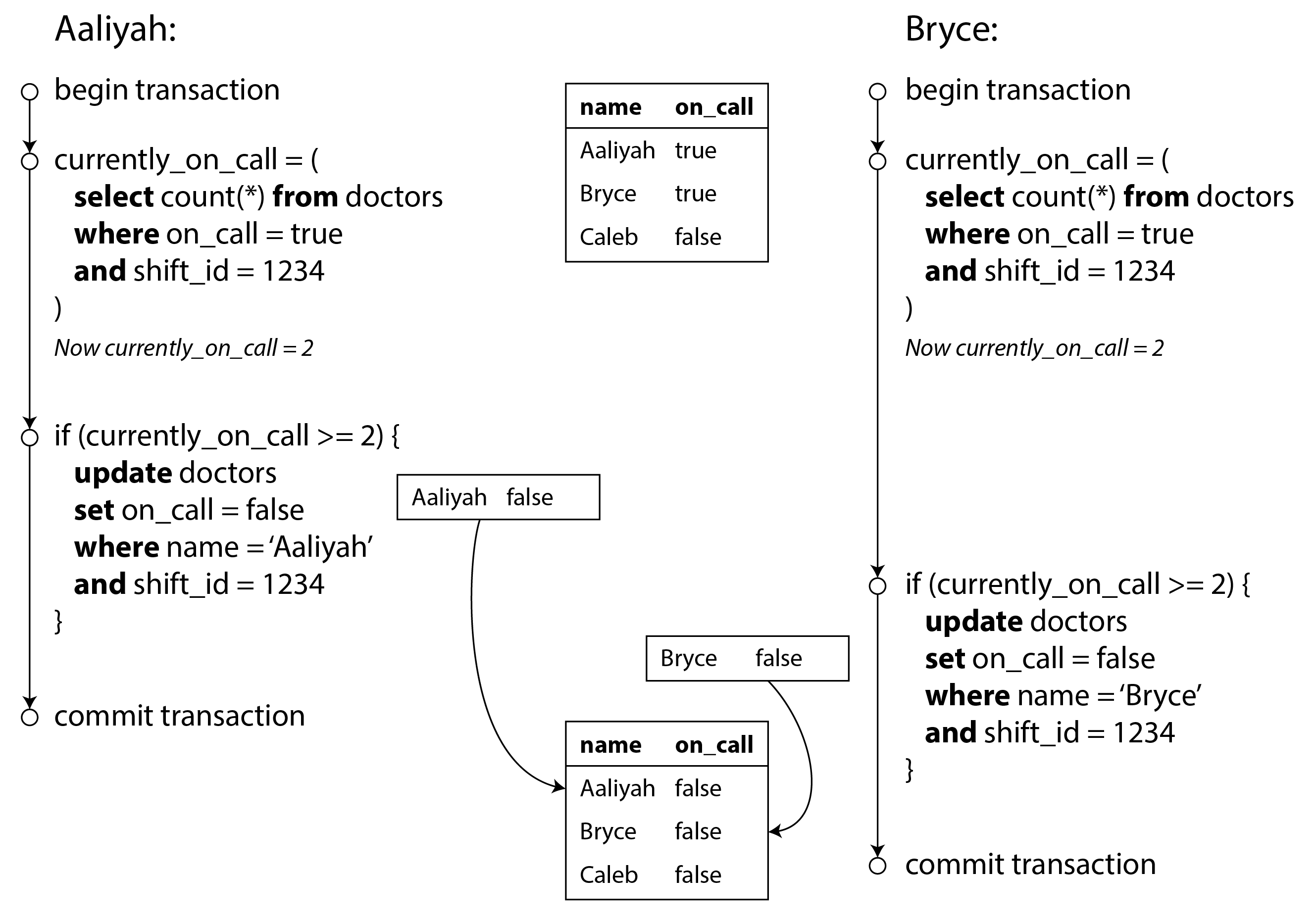
Figure 8-8 Example of write skew causing an application bug.

In each transaction, your application first checks that two or more doctors are currently on call; if yes, it assumes it’s safe for one doctor to go off call. Since the database is using snapshot isolation, both checks return 2, so both transactions proceed to the next stage. Aaliyah updates her own record to take herself off call, and Bryce updates his own record likewise. Both transactions commit, and now no doctor is on call. Your requirement of having at least one doctor on call has been violated.

Characterizing write skew

This anomaly is called write skew ³⁶. It is neither a dirty write nor a lost update, because the two transactions are updating two different objects (Aaliyah’s and Bryce’s on-call records, respectively). It is less obvious that a conflict occurred here, but it’s definitely a race condition: if the two transactions had run one after another, the second doctor would have been prevented from going off call. The anomalous behavior was only possible because the transactions ran concurrently.

You can think of write skew as a generalization of the lost update problem. Write skew can occur if two transactions read the same objects, and then update some of those objects (different transactions may update different objects). In the special case where different transactions update the same object, you get a dirty write or lost update anomaly (depending on the timing).

We saw that there are various different ways of preventing lost updates. With write skew, our options are more restricted:

Atomic single-object operations don’t help, as multiple objects are involved.
The automatic detection of lost updates that you find in some implementations of snapshot isolation unfortunately doesn’t help either: write skew is not automatically detected in PostgreSQL’s repeatable read, MySQL/InnoDB’s repeatable read, Oracle’s serializable, or SQL Server’s snapshot isolation level ²⁹. Automatically preventing write skew requires true serializable isolation (see “Serializability”).
Some databases allow you to configure constraints, which are then enforced by the database (e.g., uniqueness, foreign key constraints, or restrictions on a particular value). However, in order to specify that at least one doctor must be on call, you would need a constraint that involves multiple objects. Most databases do not have built-in support for such constraints, but you may be able to implement them with triggers or materialized views, as discussed in “Consistency” ¹².
If you can’t use a serializable isolation level, the second-best option in this case is probably to explicitly lock the rows that the transaction depends on. In the doctors example, you could write something like the following:

BEGIN TRANSACTION;

SELECT * FROM doctors
    WHERE on_call = true
    AND shift_id = 1234 FOR UPDATE; ❶

UPDATE doctors
   SET on_call = false
   WHERE name = 'Aaliyah'
   AND shift_id = 1234;

COMMIT;

❶: As before, FOR UPDATE tells the database to lock all rows returned by this query.

More examples of write skew

Write skew may seem like an esoteric issue at first, but once you’re aware of it, you may notice more situations in which it can occur. Here are some more examples:

Meeting room booking system

Say you want to enforce that there cannot be two bookings for the same meeting room at the same time ⁵⁵. When someone wants to make a booking, you first check for any conflicting bookings (i.e., bookings for the same room with an overlapping time range), and if none are found, you create the meeting (see Example 8-2).

Example 8-2. A meeting room booking system tries to avoid double-booking (not safe under snapshot isolation)

BEGIN TRANSACTION;
  
-- Check for any existing bookings that overlap with the period of noon-1pm
SELECT COUNT(*) FROM bookings
WHERE room_id = 123 AND
end_time > '2025-01-01 12:00' AND start_time < '2025-01-01 13:00';
  
-- If the previous query returned zero:
INSERT INTO bookings (room_id, start_time, end_time, user_id)
VALUES (123, '2025-01-01 12:00', '2025-01-01 13:00', 666);
  
COMMIT;

Unfortunately, snapshot isolation does not prevent another user from concurrently inserting a conflicting meeting. In order to guarantee you won’t get scheduling conflicts, you once again need serializable isolation.

Multiplayer game

In Example 8-1, we used a lock to prevent lost updates (that is, making sure that two players can’t move the same figure at the same time). However, the lock doesn’t prevent players from moving two different figures to the same position on the board or potentially making some other move that violates the rules of the game. Depending on the kind of rule you are enforcing, you might be able to use a unique constraint, but otherwise you’re vulnerable to write skew.

Claiming a username

On a website where each user has a unique username, two users may try to create accounts with the same username at the same time. You may use a transaction to check whether a name is taken and, if not, create an account with that name. However, like in the previous examples, that is not safe under snapshot isolation. Fortunately, a unique constraint is a simple solution here (the second transaction that tries to register the username will be aborted due to violating the constraint).

Preventing double-spending

A service that allows users to spend money or points needs to check that a user doesn’t spend more than they have. You might implement this by inserting a tentative spending item into a user’s account, listing all the items in the account, and checking that the sum is positive. With write skew, it could happen that two spending items are inserted concurrently that together cause the balance to go negative, but that neither transaction notices the other.

Phantoms causing write skew

All of these examples follow a similar pattern:

A SELECT query checks whether some requirement is satisfied by searching for rows that match some search condition (there are at least two doctors on call, there are no existing bookings for that room at that time, the position on the board doesn’t already have another figure on it, the username isn’t already taken, there is still money in the account).
Depending on the result of the first query, the application code decides how to continue (perhaps to go ahead with the operation, or perhaps to report an error to the user and abort).
If the application decides to go ahead, it makes a write (INSERT, UPDATE, or DELETE) to the database and commits the transaction.

The effect of this write changes the precondition of the decision of step 2. In other words, if you were to repeat the SELECT query from step 1 after committing the write, you would get a different result, because the write changed the set of rows matching the search condition (there is now one fewer doctor on call, the meeting room is now booked for that time, the position on the board is now taken by the figure that was moved, the username is now taken, there is now less money in the account).

The steps may occur in a different order. For example, you could first make the write, then the SELECT query, and finally decide whether to abort or commit based on the result of the query.

In the case of the doctor on call example, the row being modified in step 3 was one of the rows returned in step 1, so we could make the transaction safe and avoid write skew by locking the rows in step 1 (SELECT FOR UPDATE). However, the other four examples are different: they check for the absence of rows matching some search condition, and the write adds a row matching the same condition. If the query in step 1 doesn’t return any rows, SELECT FOR UPDATE can’t attach locks to anything ⁵⁶.

This effect, where a write in one transaction changes the result of a search query in another transaction, is called a phantom ⁴. Snapshot isolation avoids phantoms in read-only queries, but in read-write transactions like the examples we discussed, phantoms can lead to particularly tricky cases of write skew. The SQL generated by ORMs is also prone to write skew ⁵⁰ ⁵¹.

Materializing conflicts

If the problem of phantoms is that there is no object to which we can attach the locks, perhaps we can artificially introduce a lock object into the database?

For example, in the meeting room booking case you could imagine creating a table of time slots and rooms. Each row in this table corresponds to a particular room for a particular time period (say, 15 minutes). You create rows for all possible combinations of rooms and time periods ahead of time, e.g. for the next six months.

Now a transaction that wants to create a booking can lock (SELECT FOR UPDATE) the rows in the table that correspond to the desired room and time period. After it has acquired the locks, it can check for overlapping bookings and insert a new booking as before. Note that the additional table isn’t used to store information about the booking—it’s purely a collection of locks which is used to prevent bookings on the same room and time range from being modified concurrently.

This approach is called materializing conflicts, because it takes a phantom and turns it into a lock conflict on a concrete set of rows that exist in the database ¹⁴. Unfortunately, it can be hard and error-prone to figure out how to materialize conflicts, and it’s ugly to let a concurrency control mechanism leak into the application data model. For those reasons, materializing conflicts should be considered a last resort if no alternative is possible. A serializable isolation level is much preferable in most cases.

Serializability

In this chapter we have seen several examples of transactions that are prone to race conditions. Some race conditions are prevented by the read committed and snapshot isolation levels, but others are not. We encountered some particularly tricky examples with write skew and phantoms. It’s a sad situation:

Isolation levels are hard to understand, and inconsistently implemented in different databases (e.g., the meaning of “repeatable read” varies significantly).
If you look at your application code, it’s difficult to tell whether it is safe to run at a particular isolation level—especially in a large application, where you might not be aware of all the things that may be happening concurrently.
There are no good tools to help us detect race conditions. In principle, static analysis may help ³³, but research techniques have not yet found their way into practical use. Testing for concurrency issues is hard, because they are usually nondeterministic—problems only occur if you get unlucky with the timing.

This is not a new problem—it has been like this since the 1970s, when weak isolation levels were first introduced ³. All along, the answer from researchers has been simple: use serializable isolation!

Serializable isolation is the strongest isolation level. It guarantees that even though transactions may execute in parallel, the end result is the same as if they had executed one at a time, serially, without any concurrency. Thus, the database guarantees that if the transactions behave correctly when run individually, they continue to be correct when run concurrently—in other words, the database prevents all possible race conditions.

But if serializable isolation is so much better than the mess of weak isolation levels, then why isn’t everyone using it? To answer this question, we need to look at the options for implementing serializability, and how they perform. Most databases that provide serializability today use one of three techniques, which we will explore in the rest of this chapter:

Literally executing transactions in a serial order (see “Actual Serial Execution”)
Two-phase locking (see “Two-Phase Locking (2PL)”), which for several decades was the only viable option
Optimistic concurrency control techniques such as serializable snapshot isolation (see “Serializable Snapshot Isolation (SSI)”)

Actual Serial Execution

The simplest way of avoiding concurrency problems is to remove the concurrency entirely: to execute only one transaction at a time, in serial order, on a single thread. By doing so, we completely sidestep the problem of detecting and preventing conflicts between transactions: the resulting isolation is by definition serializable.

Even though this seems like an obvious idea, it was only in the 2000s that database designers decided that a single-threaded loop for executing transactions was feasible ⁵⁷. If multi-threaded concurrency was considered essential for getting good performance during the previous 30 years, what changed to make single-threaded execution possible?

Two developments caused this rethink:

RAM became cheap enough that for many use cases it is now feasible to keep the entire active dataset in memory (see “Keeping everything in memory”). When all data that a transaction needs to access is in memory, transactions can execute much faster than if they have to wait for data to be loaded from disk.
Database designers realized that OLTP transactions are usually short and only make a small number of reads and writes (see “Analytical versus Operational Systems”). By contrast, long-running analytic queries are typically read-only, so they can be run on a consistent snapshot (using snapshot isolation) outside of the serial execution loop.

The approach of executing transactions serially is implemented in VoltDB/H-Store, Redis, and Datomic, for example ⁵⁸ ⁵⁹ ⁶⁰. A system designed for single-threaded execution can sometimes perform better than a system that supports concurrency, because it can avoid the coordination overhead of locking. However, its throughput is limited to that of a single CPU core. In order to make the most of that single thread, transactions need to be structured differently from their traditional form.

Encapsulating transactions in stored procedures

In the early days of databases, the intention was that a database transaction could encompass an entire flow of user activity. For example, booking an airline ticket is a multi-stage process (searching for routes, fares, and available seats; deciding on an itinerary; booking seats on each of the flights of the itinerary; entering passenger details; making payment). Database designers thought that it would be neat if that entire process was one transaction so that it could be committed atomically.

Unfortunately, humans are very slow to make up their minds and respond. If a database transaction needs to wait for input from a user, the database needs to support a potentially huge number of concurrent transactions, most of them idle. Most databases cannot do that efficiently, and so almost all OLTP applications keep transactions short by avoiding interactively waiting for a user within a transaction. On the web, this means that a transaction is committed within the same HTTP request—a transaction does not span multiple requests. A new HTTP request starts a new transaction.

Even though the human has been taken out of the critical path, transactions have continued to be executed in an interactive client/server style, one statement at a time. An application makes a query, reads the result, perhaps makes another query depending on the result of the first query, and so on. The queries and results are sent back and forth between the application code (running on one machine) and the database server (on another machine).

In this interactive style of transaction, a lot of time is spent in network communication between the application and the database. If you were to disallow concurrency in the database and only process one transaction at a time, the throughput would be dreadful because the database would spend most of its time waiting for the application to issue the next query for the current transaction. In this kind of database, it’s necessary to process multiple transactions concurrently in order to get reasonable performance.

For this reason, systems with single-threaded serial transaction processing don’t allow interactive multi-statement transactions. Instead, the application must either limit itself to transactions containing a single statement, or submit the entire transaction code to the database ahead of time, as a stored procedure ⁶¹.

The differences between interactive transactions and stored procedures is illustrated in Figure 8-9. Provided that all data required by a transaction is in memory, the stored procedure can execute very quickly, without waiting for any network or disk I/O.

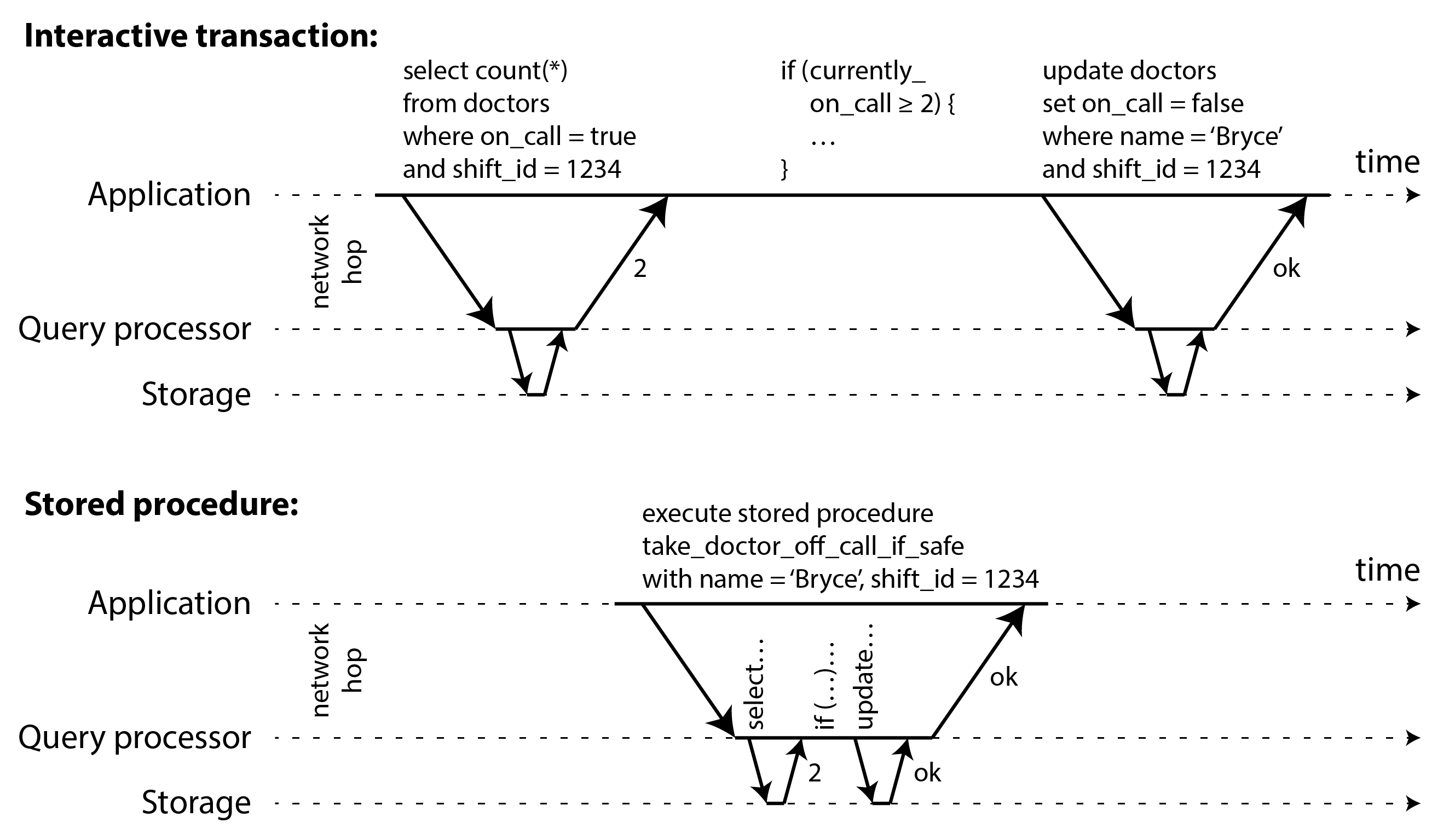
Figure 8-9 The difference between an interactive transaction and a stored procedure (using the example transaction of Figure 8-8).

Pros and cons of stored procedures

Stored procedures have existed for some time in relational databases, and they have been part of the SQL standard (SQL/PSM) since 1999. They have gained a somewhat bad reputation, for various reasons:

Traditionally, each database vendor had its own language for stored procedures (Oracle has PL/SQL, SQL Server has T-SQL, PostgreSQL has PL/pgSQL, etc.). These languages haven’t kept up with developments in general-purpose programming languages, so they look quite ugly and archaic from today’s point of view, and they lack the ecosystem of libraries that you find with most programming languages.
Code running in a database is difficult to manage: compared to an application server, it’s harder to debug, more awkward to keep in version control and deploy, trickier to test, and difficult to integrate with a metrics collection system for monitoring.
A database is often much more performance-sensitive than an application server, because a single database instance is often shared by many application servers. A badly written stored procedure (e.g., using a lot of memory or CPU time) in a database can cause much more trouble than equivalent badly written code in an application server.
In a multitenant system that allows tenants to write their own stored procedures, it’s a security risk to execute untrusted code in the same process as the database kernel ⁶².

However, those issues can be overcome. Modern implementations of stored procedures have abandoned PL/SQL and use existing general-purpose programming languages instead: VoltDB uses Java or Groovy, Datomic uses Java or Clojure, Redis uses Lua, and MongoDB uses Javascript.

Stored procedures are also useful in cases where application logic can’t easily be embedded elsewhere. Applications that use GraphQL, for example, might directly expose their database through a GraphQL proxy. If the proxy doesn’t support complex validation logic, you can embed such logic directly in the database using a stored procedure. If the database doesn’t support stored procedures, you would have to deploy a validation service between the proxy and the database to do validation.

With stored procedures and in-memory data, executing all transactions on a single thread becomes feasible. When stored procedures don’t need to wait for I/O and avoid the overhead of other concurrency control mechanisms, they can achieve quite good throughput on a single thread.

VoltDB also uses stored procedures for replication: instead of copying a transaction’s writes from one node to another, it executes the same stored procedure on each replica. VoltDB therefore requires that stored procedures are deterministic (when run on different nodes, they must produce the same result). If a transaction needs to use the current date and time, for example, it must do so through special deterministic APIs (see “Durable Execution and Workflows” for more details on deterministic operations). This approach is called state machine replication, and we will return to it in Chapter 10.

Sharding

Executing all transactions serially makes concurrency control much simpler, but limits the transaction throughput of the database to the speed of a single CPU core on a single machine. Read-only transactions may execute elsewhere, using snapshot isolation, but for applications with high write throughput, the single-threaded transaction processor can become a serious bottleneck.

In order to scale to multiple CPU cores, and multiple nodes, you can shard your data (see Chapter 7), which is supported in VoltDB. If you can find a way of sharding your dataset so that each transaction only needs to read and write data within a single shard, then each shard can have its own transaction processing thread running independently from the others. In this case, you can give each CPU core its own shard, which allows your transaction throughput to scale linearly with the number of CPU cores ⁵⁹.

However, for any transaction that needs to access multiple shards, the database must coordinate the transaction across all the shards that it touches. The stored procedure needs to be performed in lock-step across all shards to ensure serializability across the whole system.

Since cross-shard transactions have additional coordination overhead, they are vastly slower than single-shard transactions. VoltDB reports a throughput of about 1,000 cross-shard writes per second, which is orders of magnitude below its single-shard throughput and cannot be increased by adding more machines ⁶¹. More recent research has explored ways of making multi-shard transactions more scalable ⁶³.

Whether transactions can be single-shard depends very much on the structure of the data used by the application. Simple key-value data can often be sharded very easily, but data with multiple secondary indexes is likely to require a lot of cross-shard coordination (see “Sharding and Secondary Indexes”).

Summary of serial execution

Serial execution of transactions has become a viable way of achieving serializable isolation within certain constraints:

Every transaction must be small and fast, because it takes only one slow transaction to stall all transaction processing.
It is most appropriate in situations where the active dataset can fit in memory. Rarely accessed data could potentially be moved to disk, but if it needed to be accessed in a single-threaded transaction, the system would get very slow.
Write throughput must be low enough to be handled on a single CPU core, or else transactions need to be sharded without requiring cross-shard coordination.
Cross-shard transactions are possible, but their throughput is hard to scale.

Two-Phase Locking (2PL)

For around 30 years, there was only one widely used algorithm for serializability in databases: two-phase locking (2PL), sometimes called strong strict two-phase locking (SS2PL) to distinguish it from other variants of 2PL.

2PL IS NOT 2PC

Two-phase locking (2PL) and two-phase commit (2PC) are two very different things. 2PL provides serializable isolation, whereas 2PC provides atomic commit in a distributed database (see “Two-Phase Commit (2PC)”). To avoid confusion, it’s best to think of them as entirely separate concepts and to ignore the unfortunate similarity in the names.

We saw previously that locks are often used to prevent dirty writes (see “No dirty writes”): if two transactions concurrently try to write to the same object, the lock ensures that the second writer must wait until the first one has finished its transaction (aborted or committed) before it may continue.

Two-phase locking is similar, but makes the lock requirements much stronger. Several transactions are allowed to concurrently read the same object as long as nobody is writing to it. But as soon as anyone wants to write (modify or delete) an object, exclusive access is required:

If transaction A has read an object and transaction B wants to write to that object, B must wait until A commits or aborts before it can continue. (This ensures that B can’t change the object unexpectedly behind A’s back.)
If transaction A has written an object and transaction B wants to read that object, B must wait until A commits or aborts before it can continue. (Reading an old version of the object, like in Figure 8-4, is not acceptable under 2PL.)

In 2PL, writers don’t just block other writers; they also block readers and vice versa. Snapshot isolation has the mantra readers never block writers, and writers never block readers (see “Multi-version concurrency control (MVCC)”), which captures this key difference between snapshot isolation and two-phase locking. On the other hand, because 2PL provides serializability, it protects against all the race conditions discussed earlier, including lost updates and write skew.

Implementation of two-phase locking

2PL is used by the serializable isolation level in MySQL (InnoDB) and SQL Server, and the repeatable read isolation level in Db2 ²⁹.

The blocking of readers and writers is implemented by having a lock on each object in the database. The lock can either be in shared mode or in exclusive mode (also known as a multi-reader single-writer lock). The lock is used as follows:

If a transaction wants to read an object, it must first acquire the lock in shared mode. Several transactions are allowed to hold the lock in shared mode simultaneously, but if another transaction already has an exclusive lock on the object, these transactions must wait.
If a transaction wants to write to an object, it must first acquire the lock in exclusive mode. No other transaction may hold the lock at the same time (either in shared or in exclusive mode), so if there is any existing lock on the object, the transaction must wait.
If a transaction first reads and then writes an object, it may upgrade its shared lock to an exclusive lock. The upgrade works the same as getting an exclusive lock directly.
After a transaction has acquired the lock, it must continue to hold the lock until the end of the transaction (commit or abort). This is where the name “two-phase” comes from: the first phase (while the transaction is executing) is when the locks are acquired, and the second phase (at the end of the transaction) is when all the locks are released.

Since so many locks are in use, it can happen quite easily that transaction A is stuck waiting for transaction B to release its lock, and vice versa. This situation is called deadlock. The database automatically detects deadlocks between transactions and aborts one of them so that the others can make progress. The aborted transaction needs to be retried by the application.

Performance of two-phase locking

The big downside of two-phase locking, and the reason why it hasn’t been used by everybody since the 1970s, is performance: transaction throughput and response times of queries are significantly worse under two-phase locking than under weak isolation.

This is partly due to the overhead of acquiring and releasing all those locks, but more importantly due to reduced concurrency. By design, if two concurrent transactions try to do anything that may in any way result in a race condition, one has to wait for the other to complete.

For example, if you have a transaction that needs to read an entire table (e.g. a backup, analytics query, or integrity check, as discussed in “Snapshot Isolation and Repeatable Read”), that transaction has to take a shared lock on the entire table. Therefore, the reading transaction first has to wait until all in-progress transactions writing to that table have completed; then, while the whole table is being read (which may take a long time on a large table), all other transactions that want to write to that table are blocked until the big read-only transaction commits. In effect, the database becomes unavailable for writes for an extended time.

For this reason, databases running 2PL can have quite unstable latencies, and they can be very slow at high percentiles (see “Describing Performance”) if there is contention in the workload. It may take just one slow transaction, or one transaction that accesses a lot of data and acquires many locks, to cause the rest of the system to grind to a halt.

Although deadlocks can happen with the lock-based read committed isolation level, they occur much more frequently under 2PL serializable isolation (depending on the access patterns of your transaction). This can be an additional performance problem: when a transaction is aborted due to deadlock and is retried, it needs to do its work all over again. If deadlocks are frequent, this can mean significant wasted effort.

Predicate locks

In the preceding description of locks, we glossed over a subtle but important detail. In “Phantoms causing write skew” we discussed the problem of phantoms—that is, one transaction changing the results of another transaction’s search query. A database with serializable isolation must prevent phantoms.

In the meeting room booking example this means that if one transaction has searched for existing bookings for a room within a certain time window (see Example 8-2), another transaction is not allowed to concurrently insert or update another booking for the same room and time range. (It’s okay to concurrently insert bookings for other rooms, or for the same room at a different time that doesn’t affect the proposed booking.)

How do we implement this? Conceptually, we need a predicate lock ⁴. It works similarly to the shared/exclusive lock described earlier, but rather than belonging to a particular object (e.g., one row in a table), it belongs to all objects that match some search condition, such as:

SELECT * FROM bookings
 WHERE room_id = 123 AND
 end_time > '2025-01-01 12:00' AND
 start_time < '2025-01-01 13:00';

A predicate lock restricts access as follows:

If transaction A wants to read objects matching some condition, like in that SELECT query, it must acquire a shared-mode predicate lock on the conditions of the query. If another transaction B currently has an exclusive lock on any object matching those conditions, A must wait until B releases its lock before it is allowed to make its query.
If transaction A wants to insert, update, or delete any object, it must first check whether either the old or the new value matches any existing predicate lock. If there is a matching predicate lock held by transaction B, then A must wait until B has committed or aborted before it can continue.

The key idea here is that a predicate lock applies even to objects that do not yet exist in the database, but which might be added in the future (phantoms). If two-phase locking includes predicate locks, the database prevents all forms of write skew and other race conditions, and so its isolation becomes serializable.

Index-range locks

Unfortunately, predicate locks do not perform well: if there are many locks by active transactions, checking for matching locks becomes time-consuming. For that reason, most databases with 2PL actually implement index-range locking (also known as next-key locking), which is a simplified approximation of predicate locking ⁵⁴ ⁶⁴.

It’s safe to simplify a predicate by making it match a greater set of objects. For example, if you have a predicate lock for bookings of room 123 between noon and 1 p.m., you can approximate it by locking bookings for room 123 at any time, or you can approximate it by locking all rooms (not just room 123) between noon and 1 p.m. This is safe because any write that matches the original predicate will definitely also match the approximations.

In the room bookings database you would probably have an index on the room_id column, and/or indexes on start_time and end_time (otherwise the preceding query would be very slow on a large database):

Say your index is on room_id, and the database uses this index to find existing bookings for room 123. Now the database can simply attach a shared lock to this index entry, indicating that a transaction has searched for bookings of room 123.
Alternatively, if the database uses a time-based index to find existing bookings, it can attach a shared lock to a range of values in that index, indicating that a transaction has searched for bookings that overlap with the time period of noon to 1 p.m. on January 1, 2025.

Either way, an approximation of the search condition is attached to one of the indexes. Now, if another transaction wants to insert, update, or delete a booking for the same room and/or an overlapping time period, it will have to update the same part of the index. In the process of doing so, it will encounter the shared lock, and it will be forced to wait until the lock is released.

This provides effective protection against phantoms and write skew. Index-range locks are not as precise as predicate locks would be (they may lock a bigger range of objects than is strictly necessary to maintain serializability), but since they have much lower overheads, they are a good compromise.

If there is no suitable index where a range lock can be attached, the database can fall back to a shared lock on the entire table. This will not be good for performance, since it will stop all other transactions writing to the table, but it’s a safe fallback position.

Serializable Snapshot Isolation (SSI)

This chapter has painted a bleak picture of concurrency control in databases. On the one hand, we have implementations of serializability that don’t perform well (two-phase locking) or don’t scale well (serial execution). On the other hand, we have weak isolation levels that have good performance, but are prone to various race conditions (lost updates, write skew, phantoms, etc.). Are serializable isolation and good performance fundamentally at odds with each other?

It seems not: an algorithm called serializable snapshot isolation (SSI) provides full serializability with only a small performance penalty compared to snapshot isolation. SSI is comparatively new: it was first described in 2008 ⁵³ ⁶⁵.

Today SSI and similar algorithms are used in single-node databases (the serializable isolation level in PostgreSQL ⁵⁴, SQL Server’s In-Memory OLTP/Hekaton ⁶⁶, and HyPer ⁶⁷), distributed databases (CockroachDB ⁵ and FoundationDB ⁸), and embedded storage engines such as BadgerDB.

Pessimistic versus optimistic concurrency control

Two-phase locking is a so-called pessimistic concurrency control mechanism: it is based on the principle that if anything might possibly go wrong (as indicated by a lock held by another transaction), it’s better to wait until the situation is safe again before doing anything. It is like mutual exclusion, which is used to protect data structures in multi-threaded programming.

Serial execution is, in a sense, pessimistic to the extreme: it is essentially equivalent to each transaction having an exclusive lock on the entire database (or one shard of the database) for the duration of the transaction. We compensate for the pessimism by making each transaction very fast to execute, so it only needs to hold the “lock” for a short time.

By contrast, serializable snapshot isolation is an optimistic concurrency control technique. Optimistic in this context means that instead of blocking if something potentially dangerous happens, transactions continue anyway, in the hope that everything will turn out all right. When a transaction wants to commit, the database checks whether anything bad happened (i.e., whether isolation was violated); if so, the transaction is aborted and has to be retried. Only transactions that executed serializably are allowed to commit.

Optimistic concurrency control is an old idea ⁶⁸, and its advantages and disadvantages have been debated for a long time ⁶⁹. It performs badly if there is high contention (many transactions trying to access the same objects), as this leads to a high proportion of transactions needing to abort. If the system is already close to its maximum throughput, the additional transaction load from retried transactions can make performance worse.

However, if there is enough spare capacity, and if contention between transactions is not too high, optimistic concurrency control techniques tend to perform better than pessimistic ones. Contention can be reduced with commutative atomic operations: for example, if several transactions concurrently want to increment a counter, it doesn’t matter in which order the increments are applied (as long as the counter isn’t read in the same transaction), so the concurrent increments can all be applied without conflicting.

As the name suggests, SSI is based on snapshot isolation—that is, all reads within a transaction are made from a consistent snapshot of the database (see “Snapshot Isolation and Repeatable Read”). On top of snapshot isolation, SSI adds an algorithm for detecting serialization conflicts among reads and writes, and determining which transactions to abort.

Decisions based on an outdated premise

When we previously discussed write skew in snapshot isolation (see “Write Skew and Phantoms”), we observed a recurring pattern: a transaction reads some data from the database, examines the result of the query, and decides to take some action (write to the database) based on the result that it saw. However, under snapshot isolation, the result from the original query may no longer be up-to-date by the time the transaction commits, because the data may have been modified in the meantime.

Put another way, the transaction is taking an action based on a premise (a fact that was true at the beginning of the transaction, e.g., “There are currently two doctors on call”). Later, when the transaction wants to commit, the original data may have changed—the premise may no longer be true.

When the application makes a query (e.g., “How many doctors are currently on call?”), the database doesn’t know how the application logic uses the result of that query. To be safe, the database needs to assume that any change in the query result (the premise) means that writes in that transaction may be invalid. In other words, there may be a causal dependency between the queries and the writes in the transaction. In order to provide serializable isolation, the database must detect situations in which a transaction may have acted on an outdated premise and abort the transaction in that case.

How does the database know if a query result might have changed? There are two cases to consider:

Detecting reads of a stale MVCC object version (uncommitted write occurred before the read)
Detecting writes that affect prior reads (the write occurs after the read)

Detecting stale MVCC reads

Recall that snapshot isolation is usually implemented by multi-version concurrency control (MVCC; see “Multi-version concurrency control (MVCC)”). When a transaction reads from a consistent snapshot in an MVCC database, it ignores writes that were made by any other transactions that hadn’t yet committed at the time when the snapshot was taken.

In Figure 8-10, transaction 43 sees Aaliyah as having on_call = true, because transaction 42 (which modified Aaliyah’s on-call status) is uncommitted. However, by the time transaction 43 wants to commit, transaction 42 has already committed. This means that the write that was ignored when reading from the consistent snapshot has now taken effect, and transaction 43’s premise is no longer true. Things get even more complicated when a writer inserts data that didn’t exist before (see “Phantoms causing write skew”). We’ll discuss detecting phantom writes for SSI in “Detecting writes that affect prior reads”.

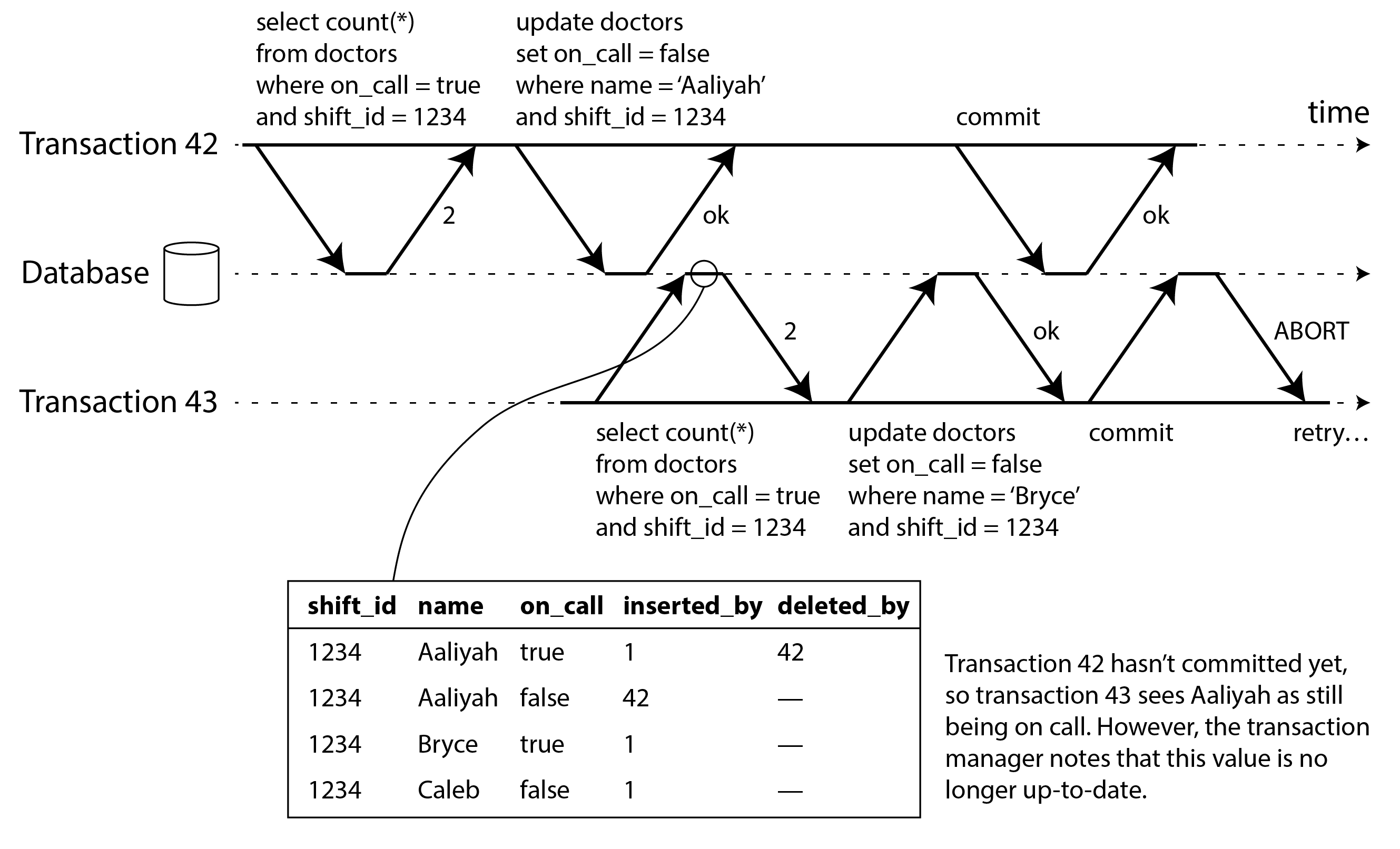
Figure 8-10 Detecting when a transaction reads outdated values from an MVCC snapshot.

In order to prevent this anomaly, the database needs to track when a transaction ignores another transaction’s writes due to MVCC visibility rules. When the transaction wants to commit, the database checks whether any of the ignored writes have now been committed. If so, the transaction must be aborted.

Why wait until committing? Why not abort transaction 43 immediately when the stale read is detected? Well, if transaction 43 was a read-only transaction, it wouldn’t need to be aborted, because there is no risk of write skew. At the time when transaction 43 makes its read, the database doesn’t yet know whether that transaction is going to later perform a write. Moreover, transaction 42 may yet abort or may still be uncommitted at the time when transaction 43 is committed, and so the read may turn out not to have been stale after all. By avoiding unnecessary aborts, SSI preserves snapshot isolation’s support for long-running reads from a consistent snapshot.

Detecting writes that affect prior reads

The second case to consider is when another transaction modifies data after it has been read. This case is illustrated in Figure 8-11.

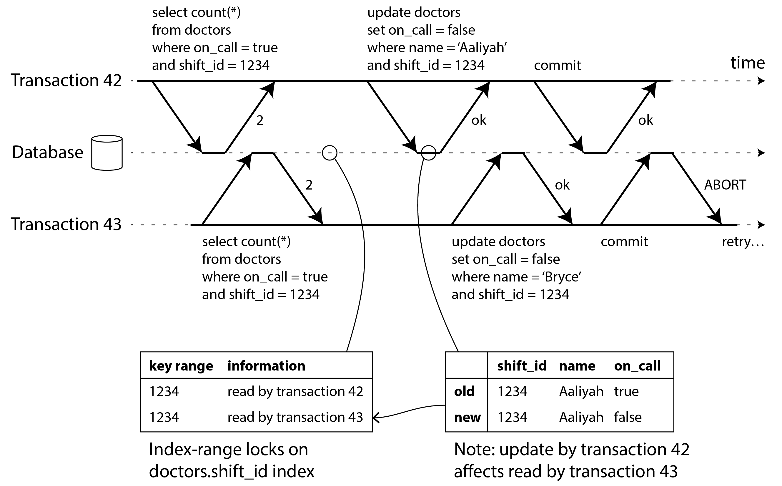
Figure 8-11 In serializable snapshot isolation, detecting when one transaction modifies another transaction's reads.

In the context of two-phase locking we discussed index-range locks (see “Index-range locks”), which allow the database to lock access to all rows matching some search query, such as WHERE shift_id = 1234. We can use a similar technique here, except that SSI locks don’t block other transactions.

In Figure 8-11, transactions 42 and 43 both search for on-call doctors during shift 1234. If there is an index on shift_id, the database can use the index entry 1234 to record the fact that transactions 42 and 43 read this data. (If there is no index, this information can be tracked at the table level.) This information only needs to be kept for a while: after a transaction has finished (committed or aborted), and all concurrent transactions have finished, the database can forget what data it read.

When a transaction writes to the database, it must look in the indexes for any other transactions that have recently read the affected data. This process is similar to acquiring a write lock on the affected key range, but rather than blocking until the readers have committed, the lock acts as a tripwire: it simply notifies the transactions that the data they read may no longer be up to date.

In Figure 8-11, transaction 43 notifies transaction 42 that its prior read is outdated, and vice versa. Transaction 42 is first to commit, and it is successful: although transaction 43’s write affected 42, 43 hasn’t yet committed, so the write has not yet taken effect. However, when transaction 43 wants to commit, the conflicting write from 42 has already been committed, so 43 must abort.

Performance of serializable snapshot isolation

As always, many engineering details affect how well an algorithm works in practice. For example, one trade-off is the granularity at which transactions’ reads and writes are tracked. If the database keeps track of each transaction’s activity in great detail, it can be precise about which transactions need to abort, but the bookkeeping overhead can become significant. Less detailed tracking is faster, but may lead to more transactions being aborted than strictly necessary.

In some cases, it’s okay for a transaction to read information that was overwritten by another transaction: depending on what else happened, it’s sometimes possible to prove that the result of the execution is nevertheless serializable. PostgreSQL uses this theory to reduce the number of unnecessary aborts ¹⁴ ⁵⁴.

Compared to two-phase locking, the big advantage of serializable snapshot isolation is that one transaction doesn’t need to block waiting for locks held by another transaction. Like under snapshot isolation, writers don’t block readers, and vice versa. This design principle makes query latency much more predictable and less variable. In particular, read-only queries can run on a consistent snapshot without requiring any locks, which is very appealing for read-heavy workloads.

Compared to serial execution, serializable snapshot isolation is not limited to the throughput of a single CPU core: for example, FoundationDB distributes the detection of serialization conflicts across multiple machines, allowing it to scale to very high throughput. Even though data may be sharded across multiple machines, transactions can read and write data in multiple shards while ensuring serializable isolation.

Compared to non-serializable snapshot isolation, the need to check for serializability violations introduces some performance overheads. How significant these overheads are is a matter of debate: some believe that serializability checking is not worth it ⁷⁰, while others believe that the performance of serializability is now so good that there is no need to use the weaker snapshot isolation any more ⁶⁷.

The rate of aborts significantly affects the overall performance of SSI. For example, a transaction that reads and writes data over a long period of time is likely to run into conflicts and abort, so SSI requires that read-write transactions be fairly short (long-running read-only transactions are okay). However, SSI is less sensitive to slow transactions than two-phase locking or serial execution.

Distributed Transactions

The last few sections have focused on concurrency control for isolation, the I in ACID. The algorithms we have seen apply to both single-node and distributed databases: although there are challenges in making concurrency control algorithms scalable (for example, performing distributed serializability checking for SSI), the high-level ideas for distributed concurrency control are similar to single-node concurrency control ⁸.

Consistency and durability also don’t change much when we move to distributed transactions. However, atomicity requires more care.

For transactions that execute at a single database node, atomicity is commonly implemented by the storage engine. When the client asks the database node to commit the transaction, the database makes the transaction’s writes durable (typically in a write-ahead log; see “Making B-trees reliable”) and then appends a commit record to the log on disk. If the database crashes in the middle of this process, the transaction is recovered from the log when the node restarts: if the commit record was successfully written to disk before the crash, the transaction is considered committed; if not, any writes from that transaction are rolled back.

Thus, on a single node, transaction commitment crucially depends on the order in which data is durably written to disk: first the data, then the commit record ²². The key deciding moment for whether the transaction commits or aborts is the moment at which the disk finishes writing the commit record: before that moment, it is still possible to abort (due to a crash), but after that moment, the transaction is committed (even if the database crashes). Thus, it is a single device (the controller of one particular disk drive, attached to one particular node) that makes the commit atomic.

However, what if multiple nodes are involved in a transaction? For example, perhaps you have a multi-object transaction in a sharded database, or a global secondary index (in which the index entry may be on a different node from the primary data; see “Sharding and Secondary Indexes”). Most “NoSQL” distributed datastores do not support such distributed transactions, but various distributed relational databases do.

In these cases, it is not sufficient to simply send a commit request to all of the nodes and independently commit the transaction on each one. It could easily happen that the commit succeeds on some nodes and fails on other nodes, as shown in Figure 8-12:

Some nodes may detect a constraint violation or conflict, making an abort necessary, while other nodes are successfully able to commit.
Some of the commit requests might be lost in the network, eventually aborting due to a timeout, while other commit requests get through.
Some nodes may crash before the commit record is fully written and roll back on recovery, while others successfully commit.

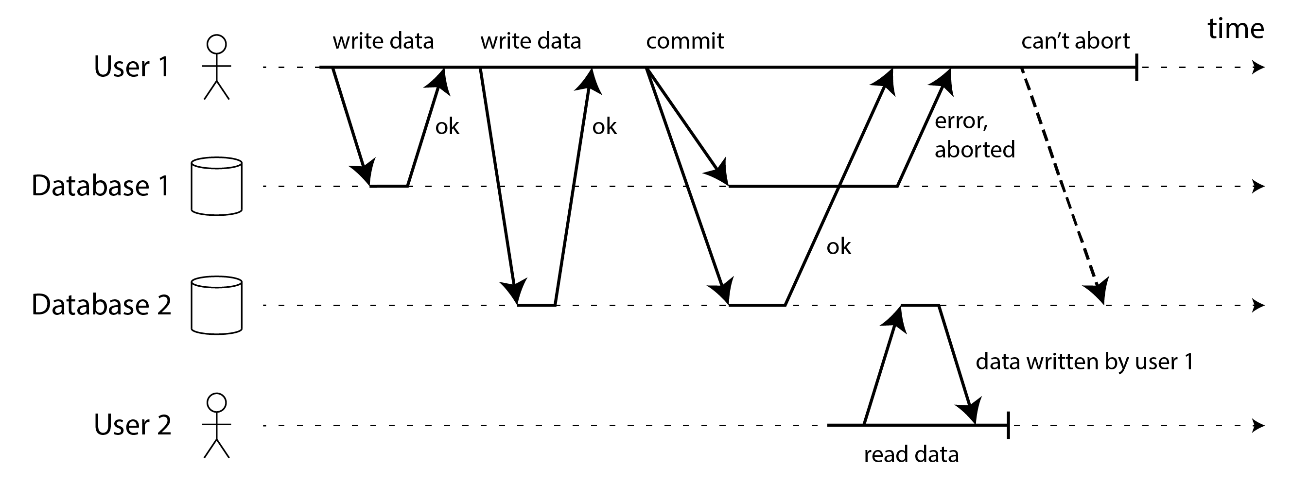
Figure 8-12 When a transaction involves multiple database nodes, it may commit on some and fail on others.

If some nodes commit the transaction but others abort it, the nodes become inconsistent with each other. And once a transaction has been committed on one node, it cannot be retracted again if it later turns out that it was aborted on another node. This is because once data has been committed, it becomes visible to other transactions under read committed or stronger isolation. For example, in Figure 8-12, by the time user 1 notices that its commit failed on database 1, user 2 has already read the data from the same transaction on database 2. If user 1’s transaction was later aborted, user 2’s transaction would have to be reverted as well, since it was based on data that was retroactively declared not to have existed.

A better approach is to ensure that the nodes involved in a transaction either all commit or all abort, and to prevent a mixture of the two. Ensuring this is known as the atomic commitment problem.

Two-Phase Commit (2PC)

Two-phase commit is an algorithm for achieving atomic transaction commit across multiple nodes. It is a classic algorithm in distributed databases ¹³ ⁷¹ ⁷². 2PC is used internally in some databases and also made available to applications in the form of XA transactions ⁷³ (which are supported by the Java Transaction API, for example) or via WS-AtomicTransaction for SOAP web services ⁷⁴ ⁷⁵.

The basic flow of 2PC is illustrated in Figure 8-13. Instead of a single commit request, as with a single-node transaction, the commit/abort process in 2PC is split into two phases (hence the name).

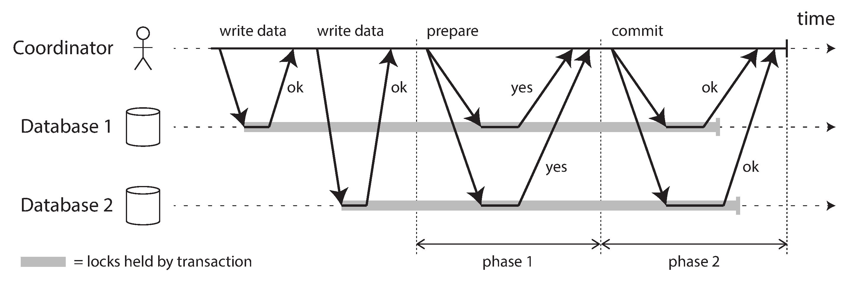
Figure 8-13 A successful execution of two-phase commit (2PC).

2PC uses a new component that does not normally appear in single-node transactions: a coordinator (also known as transaction manager). The coordinator is often implemented as a library within the same application process that is requesting the transaction (e.g., embedded in a Java EE container), but it can also be a separate process or service. Examples of such coordinators include Narayana, JOTM, BTM, or MSDTC.

When 2PC is used, a distributed transaction begins with the application reading and writing data on multiple database nodes, as normal. We call these database nodes participants in the transaction. When the application is ready to commit, the coordinator begins phase 1: it sends a prepare request to each of the nodes, asking them whether they are able to commit. The coordinator then tracks the responses from the participants:

If all participants reply “yes,” indicating they are ready to commit, then the coordinator sends out a commit request in phase 2, and the commit actually takes place.
If any of the participants replies “no,” the coordinator sends an abort request to all nodes in phase 2.

This process is somewhat like the traditional marriage ceremony in Western cultures: the minister asks the bride and groom individually whether each wants to marry the other, and typically receives the answer “I do” from both. After receiving both acknowledgments, the minister pronounces the couple husband and wife: the transaction is committed, and the happy fact is broadcast to all attendees. If either bride or groom does not say “yes,” the ceremony is aborted ⁷⁶.

A system of promises

From this short description it might not be clear why two-phase commit ensures atomicity, while one-phase commit across several nodes does not. Surely the prepare and commit requests can just as easily be lost in the two-phase case. What makes 2PC different?

To understand why it works, we have to break down the process in a bit more detail:

When the application wants to begin a distributed transaction, it requests a transaction ID from the coordinator. This transaction ID is globally unique.
The application begins a single-node transaction on each of the participants, and attaches the globally unique transaction ID to the single-node transaction. All reads and writes are done in one of these single-node transactions. If anything goes wrong at this stage (for example, a node crashes or a request times out), the coordinator or any of the participants can abort.
When the application is ready to commit, the coordinator sends a prepare request to all participants, tagged with the global transaction ID. If any of these requests fails or times out, the coordinator sends an abort request for that transaction ID to all participants.
When a participant receives the prepare request, it makes sure that it can definitely commit the transaction under all circumstances.

This includes writing all transaction data to disk (a crash, a power failure, or running out of disk space is not an acceptable excuse for refusing to commit later), and checking for any conflicts or constraint violations. By replying “yes” to the coordinator, the node promises to commit the transaction without error if requested. In other words, the participant surrenders the right to abort the transaction, but without actually committing it. 5. When the coordinator has received responses to all prepare requests, it makes a definitive decision on whether to commit or abort the transaction (committing only if all participants voted “yes”). The coordinator must write that decision to its transaction log on disk so that it knows which way it decided in case it subsequently crashes. This is called the commit point. 6. Once the coordinator’s decision has been written to disk, the commit or abort request is sent to all participants. If this request fails or times out, the coordinator must retry forever until it succeeds. There is no more going back: if the decision was to commit, that decision must be enforced, no matter how many retries it takes. If a participant has crashed in the meantime, the transaction will be committed when it recovers—since the participant voted “yes,” it cannot refuse to commit when it recovers.

Thus, the protocol contains two crucial “points of no return”: when a participant votes “yes,” it promises that it will definitely be able to commit later (although the coordinator may still choose to abort); and once the coordinator decides, that decision is irrevocable. Those promises ensure the atomicity of 2PC. (Single-node atomic commit lumps these two events into one: writing the commit record to the transaction log.)

Returning to the marriage analogy, before saying “I do,” you and your bride/groom have the freedom to abort the transaction by saying “No way!” (or something to that effect). However, after saying “I do,” you cannot retract that statement. If you faint after saying “I do” and you don’t hear the minister speak the words “You are now husband and wife,” that doesn’t change the fact that the transaction was committed. When you recover consciousness later, you can find out whether you are married or not by querying the minister for the status of your global transaction ID, or you can wait for the minister’s next retry of the commit request (since the retries will have continued throughout your period of unconsciousness).

Coordinator failure

We have discussed what happens if one of the participants or the network fails during 2PC: if any of the prepare requests fails or times out, the coordinator aborts the transaction; if any of the commit or abort requests fails, the coordinator retries them indefinitely. However, it is less clear what happens if the coordinator crashes.

If the coordinator fails before sending the prepare requests, a participant can safely abort the transaction. But once the participant has received a prepare request and voted “yes,” it can no longer abort unilaterally—it must wait to hear back from the coordinator whether the transaction was committed or aborted. If the coordinator crashes or the network fails at this point, the participant can do nothing but wait. A participant’s transaction in this state is called in doubt or uncertain.

The situation is illustrated in Figure 8-14. In this particular example, the coordinator actually decided to commit, and database 2 received the commit request. However, the coordinator crashed before it could send the commit request to database 1, and so database 1 does not know whether to commit or abort. Even a timeout does not help here: if database 1 unilaterally aborts after a timeout, it will end up inconsistent with database 2, which has committed. Similarly, it is not safe to unilaterally commit, because another participant may have aborted.

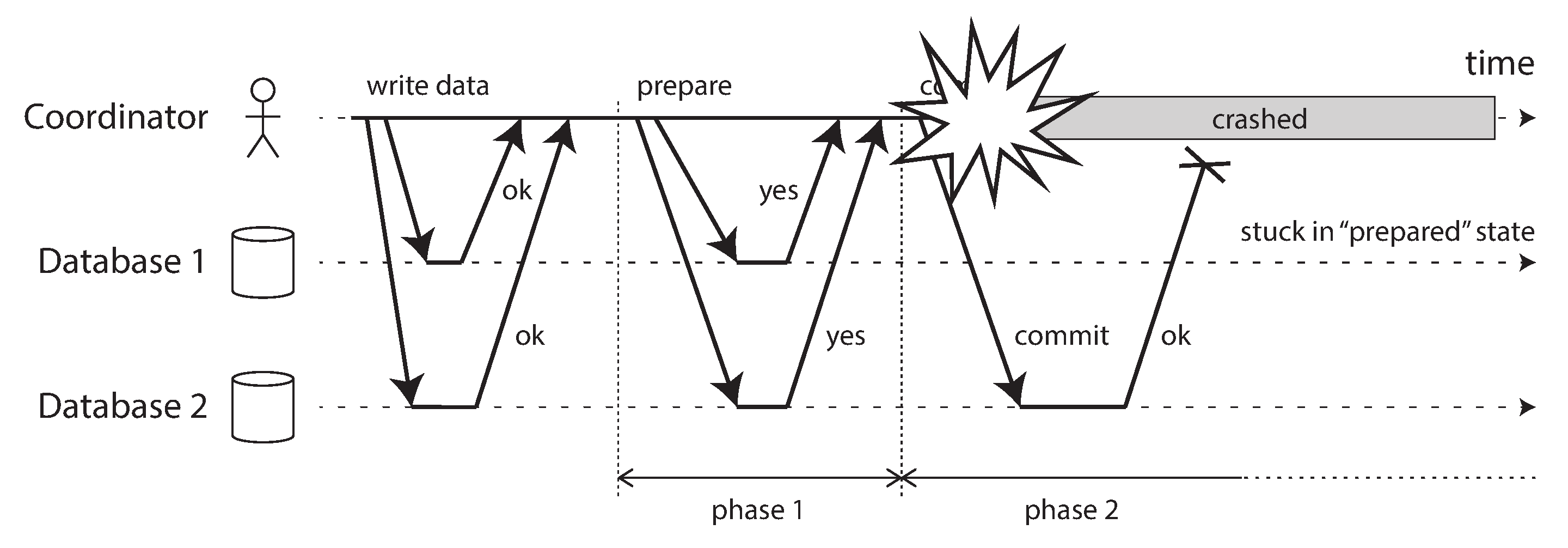
Figure 8-14 The coordinator crashes after participants vote "yes." Database 1 does not know whether to commit or abort.

Without hearing from the coordinator, the participant has no way of knowing whether to commit or abort. In principle, the participants could communicate among themselves to find out how each participant voted and come to some agreement, but that is not part of the 2PC protocol.

The only way 2PC can complete is by waiting for the coordinator to recover. This is why the coordinator must write its commit or abort decision to a transaction log on disk before sending commit or abort requests to participants: when the coordinator recovers, it determines the status of all in-doubt transactions by reading its transaction log. Any transactions that don’t have a commit record in the coordinator’s log are aborted. Thus, the commit point of 2PC comes down to a regular single-node atomic commit on the coordinator.

Three-phase commit

Two-phase commit is called a blocking atomic commit protocol due to the fact that 2PC can become stuck waiting for the coordinator to recover. It is possible to make an atomic commit protocol nonblocking, so that it does not get stuck if a node fails. However, making this work in practice is not so straightforward.

As an alternative to 2PC, an algorithm called three-phase commit (3PC) has been proposed ¹³ ⁷⁷. However, 3PC assumes a network with bounded delay and nodes with bounded response times; in most practical systems with unbounded network delay and process pauses (see Chapter 9), it cannot guarantee atomicity.

A better solution in practice is to replace the single-node coordinator with a fault-tolerant consensus protocol. We will see how to do this in Chapter 10.

Distributed Transactions Across Different Systems

Distributed transactions and two-phase commit have a mixed reputation. On the one hand, they are seen as providing an important safety guarantee that would be hard to achieve otherwise; on the other hand, they are criticized for causing operational problems, killing performance, and promising more than they can deliver ⁷⁸ ⁷⁹ ⁸⁰ ⁸¹. Many cloud services choose not to implement distributed transactions due to the operational problems they engender ⁸².

Some implementations of distributed transactions carry a heavy performance penalty. Much of the performance cost inherent in two-phase commit is due to the additional disk forcing (fsync) that is required for crash recovery, and the additional network round-trips.

However, rather than dismissing distributed transactions outright, we should examine them in some more detail, because there are important lessons to be learned from them. To begin, we should be precise about what we mean by “distributed transactions.” Two quite different types of distributed transactions are often conflated:

Database-internal distributed transactions: Some distributed databases (i.e., databases that use replication and sharding in their standard configuration) support internal transactions among the nodes of that database. For example, YugabyteDB, TiDB, FoundationDB, Spanner, VoltDB, and MySQL Cluster’s NDB storage engine have such internal transaction support. In this case, all the nodes participating in the transaction are running the same database software.
Heterogeneous distributed transactions: In a heterogeneous transaction, the participants are two or more different technologies: for example, two databases from different vendors, or even non-database systems such as message brokers. A distributed transaction across these systems must ensure atomic commit, even though the systems may be entirely different under the hood.

Database-internal transactions do not have to be compatible with any other system, so they can use any protocol and apply optimizations specific to that particular technology. For that reason, database-internal distributed transactions can often work quite well. On the other hand, transactions spanning heterogeneous technologies are a lot more challenging.

Exactly-once message processing

Heterogeneous distributed transactions allow diverse systems to be integrated in powerful ways. For example, a message from a message queue can be acknowledged as processed if and only if the database transaction for processing the message was successfully committed. This is implemented by atomically committing the message acknowledgment and the database writes in a single transaction. With distributed transaction support, this is possible, even if the message broker and the database are two unrelated technologies running on different machines.

If either the message delivery or the database transaction fails, both are aborted, and so the message broker may safely redeliver the message later. Thus, by atomically committing the message and the side effects of its processing, we can ensure that the message is effectively processed exactly once, even if it required a few retries before it succeeded. The abort discards any side effects of the partially completed transaction. This is known as exactly-once semantics.

Such a distributed transaction is only possible if all systems affected by the transaction are able to use the same atomic commit protocol, however. For example, say a side effect of processing a message is to send an email, and the email server does not support two-phase commit: it could happen that the email is sent two or more times if message processing fails and is retried. But if all side effects of processing a message are rolled back on transaction abort, then the processing step can safely be retried as if nothing had happened.

We will return to the topic of exactly-once semantics later in this chapter. Let’s look first at the atomic commit protocol that allows such heterogeneous distributed transactions.

XA transactions

X/Open XA (short for eXtended Architecture) is a standard for implementing two-phase commit across heterogeneous technologies ⁷³. It was introduced in 1991 and has been widely implemented: XA is supported by many traditional relational databases (including PostgreSQL, MySQL, Db2, SQL Server, and Oracle) and message brokers (including ActiveMQ, HornetQ, MSMQ, and IBM MQ).

XA is not a network protocol—it is merely a C API for interfacing with a transaction coordinator. Bindings for this API exist in other languages; for example, in the world of Java EE applications, XA transactions are implemented using the Java Transaction API (JTA), which in turn is supported by many drivers for databases using Java Database Connectivity (JDBC) and drivers for message brokers using the Java Message Service (JMS) APIs.

XA assumes that your application uses a network driver or client library to communicate with the participant databases or messaging services. If the driver supports XA, that means it calls the XA API to find out whether an operation should be part of a distributed transaction—and if so, it sends the necessary information to the database server. The driver also exposes callbacks through which the coordinator can ask the participant to prepare, commit, or abort.

The transaction coordinator implements the XA API. The standard does not specify how it should be implemented, but in practice the coordinator is often simply a library that is loaded into the same process as the application issuing the transaction (not a separate service). It keeps track of the participants in a transaction, collects partipants’ responses after asking them to prepare (via a callback into the driver), and uses a log on the local disk to keep track of the commit/abort decision for each transaction.

If the application process crashes, or the machine on which the application is running dies, the coordinator goes with it. Any participants with prepared but uncommitted transactions are then stuck in doubt. Since the coordinator’s log is on the application server’s local disk, that server must be restarted, and the coordinator library must read the log to recover the commit/abort outcome of each transaction. Only then can the coordinator use the database driver’s XA callbacks to ask participants to commit or abort, as appropriate. The database server cannot contact the coordinator directly, since all communication must go via its client library.

Holding locks while in doubt

Why do we care so much about a transaction being stuck in doubt? Can’t the rest of the system just get on with its work, and ignore the in-doubt transaction that will be cleaned up eventually?

The problem is with locking. As discussed in “Read Committed”, database transactions usually take a row-level exclusive lock on any rows they modify, to prevent dirty writes. In addition, if you want serializable isolation, a database using two-phase locking would also have to take a shared lock on any rows read by the transaction.

The database cannot release those locks until the transaction commits or aborts (illustrated as a shaded area in Figure 8-13). Therefore, when using two-phase commit, a transaction must hold onto the locks throughout the time it is in doubt. If the coordinator has crashed and takes 20 minutes to start up again, those locks will be held for 20 minutes. If the coordinator’s log is entirely lost for some reason, those locks will be held forever—or at least until the situation is manually resolved by an administrator.

While those locks are held, no other transaction can modify those rows. Depending on the isolation level, other transactions may even be blocked from reading those rows. Thus, other transactions cannot simply continue with their business—if they want to access that same data, they will be blocked. This can cause large parts of your application to become unavailable until the in-doubt transaction is resolved.

Recovering from coordinator failure

In theory, if the coordinator crashes and is restarted, it should cleanly recover its state from the log and resolve any in-doubt transactions. However, in practice, orphaned in-doubt transactions do occur ⁸³ ⁸⁴ — that is, transactions for which the coordinator cannot decide the outcome for whatever reason (e.g., because the transaction log has been lost or corrupted due to a software bug). These transactions cannot be resolved automatically, so they sit forever in the database, holding locks and blocking other transactions.

Even rebooting your database servers will not fix this problem, since a correct implementation of 2PC must preserve the locks of an in-doubt transaction even across restarts (otherwise it would risk violating the atomicity guarantee). It’s a sticky situation.

The only way out is for an administrator to manually decide whether to commit or roll back the transactions. The administrator must examine the participants of each in-doubt transaction, determine whether any participant has committed or aborted already, and then apply the same outcome to the other participants. Resolving the problem potentially requires a lot of manual effort, and most likely needs to be done under high stress and time pressure during a serious production outage (otherwise, why would the coordinator be in such a bad state?).

Many XA implementations have an emergency escape hatch called heuristic decisions: allowing a participant to unilaterally decide to abort or commit an in-doubt transaction without a definitive decision from the coordinator ⁷³. To be clear, heuristic here is a euphemism for probably breaking atomicity, since the heuristic decision violates the system of promises in two-phase commit. Thus, heuristic decisions are intended only for getting out of catastrophic situations, and not for regular use.

Problems with XA transactions

A single-node coordinator is a single point of failure for the entire system, and making it part of the application server is also problematic because the coordinator’s logs on its local disk become a crucial part of the durable system state—as important as the databases themselves.

In principle, the coordinator of an XA transaction could be highly available and replicated, just like we would expect of any other important database. Unfortunately, this still doesn’t solve a fundamental problem with XA, which is that it provides no way for the coordinator and the participants of a transaction to communicate with each other directly. They can only communicate via the application code that invoked the transaction, and the database drivers through which it calls the participants.

Even if the coordinator were replicated, the application code would therefore be a single point of failure. Solving this problem would require totally redesigning how application code is run to make it replicated or restartable, which could perhaps look similar to durable execution (see “Durable Execution and Workflows”). However, there don’t seem to be any tools that actually take this approach in practice.

Another problem is that since XA needs to be compatible with a wide range of data systems, it is necessarily a lowest common denominator. For example, it cannot detect deadlocks across different systems (since that would require a standardized protocol for systems to exchange information on the locks that each transaction is waiting for), and it does not work with SSI (see “Serializable Snapshot Isolation (SSI)”), since that would require a protocol for identifying conflicts across different systems.

These problems are somewhat inherent in performing transactions across heterogeneous technologies. However, keeping several heterogeneous data systems consistent with each other is still a real and important problem, so we need to find a different solution to it. This can be done, as we will see in the next section and in “Derived data versus distributed transactions”.

Database-internal Distributed Transactions

As explained previously, there is a big difference between distributed transactions that span multiple heterogeneous storage technologies, and those that are internal to a system—i.e., where all the participating nodes are shards of the same database running the same software. Such internal distributed transactions are a defining feature of “NewSQL” databases such as CockroachDB ⁵, TiDB ⁶, Spanner ⁷, FoundationDB ⁸, and YugabyteDB, for example. Some message brokers such as Kafka also support internal distributed transactions ⁸⁵.

Many of these systems use 2-phase commit to ensure atomicity of transactions that write to multiple shards, and yet they don’t suffer the same problems as XA transactions. The reason is that because their distributed transactions don’t need to interface with any other technologies, they avoid the lowest-common-denominator trap—the designers of these systems are free to use better protocols that are more reliable and faster.

The biggest problems with XA can be fixed by:

Replicating the coordinator, with automatic failover to another coordinator node if the primary one crashes;
Allowing the coordinator and data shards to communicate directly without going via application code;
Replicating the participating shards, so that the risk of having to abort a transaction because of a fault in one of the shards is reduced; and
Coupling the atomic commitment protocol with a distributed concurrency control protocol that supports deadlock detection and consistent reads across shards.

Consensus algorithms are commonly used to replicate the coordinator and the database shards. We will see in Chapter 10 how atomic commitment for distributed transactions can be implemented using a consensus algorithm. These algorithms tolerate faults by automatically failing over from one node to another without any human intervention, and while continuing to guarantee strong consistency properties.

The isolation levels offered for distributed transactions depend on the system, but snapshot isolation and serializable snapshot isolation are both possible across shards. The details of how this works can be found in the papers referenced at the end of this chapter.

Exactly-once message processing revisited

We saw in “Exactly-once message processing” that an important use case for distributed transactions is to ensure that some operation takes effect exactly once, even if a crash occurs while it is being processed and the processing needs to be retried. If you can atomically commit a transaction across a message broker and a database, you can acknowledge the message to the broker if and only if it was successfully processed and the database writes resulting from the process were committed.

However, you don’t actually need such distributed transactions to achieve exactly-once semantics. An alternative approach is as follows, which only requires transactions within the database:

Assume every message has a unique ID, and in the database you have a table of message IDs that have been processed. When you start processing a message from the broker, you begin a new transaction on the database, and check the message ID. If the same message ID is already present in the database, you know that it has already been processed, so you can acknowledge the message to the broker and drop it.
If the message ID is not already in the database, you add it to the table. You then process the message, which may result in additional writes to the database within the same transaction. When you finish processing the message, you commit the transaction on the database.
Once the database transaction is successfully committed, you can acknowledge the message to the broker.
Once the message has successfully been acknowledged to the broker, you know that it won’t try processing the same message again, so you can delete the message ID from the database (in a separate transaction).

If the message processor crashes before committing the database transaction, the transaction is aborted and the message broker will retry processing. If it crashes after committing but before acknowledging the message to the broker, it will also retry processing, but the retry will see the message ID in the database and drop it. If it crashes after acknowledging the message but before deleting the message ID from the database, you will have an old message ID lying around, which doesn’t do any harm besides taking a little bit of storage space. If a retry happens before the database transaction is aborted (which could happen if communication between the message processor and the database is interrupted), a uniqueness constraint on the table of message IDs should prevent the same message ID from being inserted by two concurrent transactions.

Thus, achieving exactly-once processing only requires transactions within the database—atomicity across database and message broker is not necessary for this use case. Recording the message ID in the database makes the message processing idempotent, so that message processing can be safely retried without duplicating its side-effects. A similar approach is used in stream processing frameworks such as Kafka Streams to achieve exactly-once semantics, as we shall see in “Fault Tolerance”.

However, internal distributed transactions within the database are still useful for the scalability of patterns such as these: for example, they would allow the message IDs to be stored on one shard and the main data updated by the message processing to be stored on other shards, and to ensure atomicity of the transaction commit across those shards.

Summary

Transactions are an abstraction layer that allows an application to pretend that certain concurrency problems and certain kinds of hardware and software faults don’t exist. A large class of errors is reduced down to a simple transaction abort, and the application just needs to try again.

In this chapter we saw many examples of problems that transactions help prevent. Not all applications are susceptible to all those problems: an application with very simple access patterns, such as reading and writing only a single record, can probably manage without transactions. However, for more complex access patterns, transactions can hugely reduce the number of potential error cases you need to think about.

Without transactions, various error scenarios (processes crashing, network interruptions, power outages, disk full, unexpected concurrency, etc.) mean that data can become inconsistent in various ways. For example, denormalized data can easily go out of sync with the source data. Without transactions, it becomes very difficult to reason about the effects that complex interacting accesses can have on the database.

In this chapter, we went particularly deep into the topic of concurrency control. We discussed several widely used isolation levels, in particular read committed, snapshot isolation (sometimes called repeatable read), and serializable. We characterized those isolation levels by discussing various examples of race conditions, summarized in Table 8-1:

Isolation level	Dirty reads	Read skew	Phantom reads	Lost updates	Write skew
Read uncommitted	✗ Possible	✗ Possible	✗ Possible	✗ Possible	✗ Possible
Read committed	✓ Prevented	✗ Possible	✗ Possible	✗ Possible	✗ Possible
Snapshot isolation	✓ Prevented	✓ Prevented	✓ Prevented	? Depends	✗ Possible
Serializable	✓ Prevented	✓ Prevented	✓ Prevented	✓ Prevented	✓ Prevented

Table 8-1 Summary of anomalies that can occur at various isolation levels

Dirty reads: One client reads another client’s writes before they have been committed. The read committed isolation level and stronger levels prevent dirty reads.
Dirty writes: One client overwrites data that another client has written, but not yet committed. Almost all transaction implementations prevent dirty writes.
Read skew: A client sees different parts of the database at different points in time. Some cases of read skew are also known as nonrepeatable reads. This issue is most commonly prevented with snapshot isolation, which allows a transaction to read from a consistent snapshot corresponding to one particular point in time. It is usually implemented with multi-version concurrency control (MVCC).
Lost updates: Two clients concurrently perform a read-modify-write cycle. One overwrites the other’s write without incorporating its changes, so data is lost. Some implementations of snapshot isolation prevent this anomaly automatically, while others require a manual lock (SELECT FOR UPDATE).
Write skew: A transaction reads something, makes a decision based on the value it saw, and writes the decision to the database. However, by the time the write is made, the premise of the decision is no longer true. Only serializable isolation prevents this anomaly.
Phantom reads: A transaction reads objects that match some search condition. Another client makes a write that affects the results of that search. Snapshot isolation prevents straightforward phantom reads, but phantoms in the context of write skew require special treatment, such as index-range locks.

Weak isolation levels protect against some of those anomalies but leave you, the application developer, to handle others manually (e.g., using explicit locking). Only serializable isolation protects against all of these issues. We discussed three different approaches to implementing serializable transactions:

Literally executing transactions in a serial order: If you can make each transaction very fast to execute (typically by using stored procedures), and the transaction throughput is low enough to process on a single CPU core or can be sharded, this is a simple and effective option.
Two-phase locking: For decades this has been the standard way of implementing serializability, but many applications avoid using it because of its poor performance.
Serializable snapshot isolation (SSI): A comparatively new algorithm that avoids most of the downsides of the previous approaches. It uses an optimistic approach, allowing transactions to proceed without blocking. When a transaction wants to commit, it is checked, and it is aborted if the execution was not serializable.

Finally, we examined how to achieve atomicity when a transaction is distributed across multiple nodes, using two-phase commit. If those nodes are all running the same database software, distributed transactions can work quite well, but across different storage technologies (using XA transactions), 2PC is problematic: it is very sensitive to faults in the coordinator and the application code driving the transaction, and it interacts poorly with concurrency control mechanisms. Fortunately, idempotence can ensure exactly-once semantics without requiring atomic commit across different storage technologies, and we will see more on this in later chapters.

The examples in this chapter used a relational data model. However, as discussed in “The need for multi-object transactions”, transactions are a valuable database feature, no matter which data model is used.

References

Steven J. Murdoch. What went wrong with Horizon: learning from the Post Office Trial. benthamsgaze.org, July 2021. Archived at perma.cc/CNM4-553F ↩︎
Donald D. Chamberlin, Morton M. Astrahan, Michael W. Blasgen, James N. Gray, W. Frank King, Bruce G. Lindsay, Raymond Lorie, James W. Mehl, Thomas G. Price, Franco Putzolu, Patricia Griffiths Selinger, Mario Schkolnick, Donald R. Slutz, Irving L. Traiger, Bradford W. Wade, and Robert A. Yost. A History and Evaluation of System R. Communications of the ACM, volume 24, issue 10, pages 632–646, October 1981. doi:10.1145/358769.358784 ↩︎
Jim N. Gray, Raymond A. Lorie, Gianfranco R. Putzolu, and Irving L. Traiger. Granularity of Locks and Degrees of Consistency in a Shared Data Base. in Modelling in Data Base Management Systems: Proceedings of the IFIP Working Conference on Modelling in Data Base Management Systems, edited by G. M. Nijssen, pages 364–394, Elsevier/North Holland Publishing, 1976. Also in Readings in Database Systems, 4th edition, edited by Joseph M. Hellerstein and Michael Stonebraker, MIT Press, 2005. ISBN: 978-0-262-69314-1 ↩︎ ↩︎ ↩︎ ↩︎
Kapali P. Eswaran, Jim N. Gray, Raymond A. Lorie, and Irving L. Traiger. The Notions of Consistency and Predicate Locks in a Database System. Communications of the ACM, volume 19, issue 11, pages 624–633, November 1976. doi:10.1145/360363.360369 ↩︎ ↩︎ ↩︎
Rebecca Taft, Irfan Sharif, Andrei Matei, Nathan VanBenschoten, Jordan Lewis, Tobias Grieger, Kai Niemi, Andy Woods, Anne Birzin, Raphael Poss, Paul Bardea, Amruta Ranade, Ben Darnell, Bram Gruneir, Justin Jaffray, Lucy Zhang, and Peter Mattis. CockroachDB: The Resilient Geo-Distributed SQL Database. At ACM SIGMOD International Conference on Management of Data (SIGMOD), pages 1493–1509, June 2020. doi:10.1145/3318464.3386134 ↩︎ ↩︎ ↩︎
Dongxu Huang, Qi Liu, Qiu Cui, Zhuhe Fang, Xiaoyu Ma, Fei Xu, Li Shen, Liu Tang, Yuxing Zhou, Menglong Huang, Wan Wei, Cong Liu, Jian Zhang, Jianjun Li, Xuelian Wu, Lingyu Song, Ruoxi Sun, Shuaipeng Yu, Lei Zhao, Nicholas Cameron, Liquan Pei, and Xin Tang. TiDB: a Raft-based HTAP database. Proceedings of the VLDB Endowment, volume 13, issue 12, pages 3072–3084. doi:10.14778/3415478.3415535 ↩︎ ↩︎
James C. Corbett, Jeffrey Dean, Michael Epstein, Andrew Fikes, Christopher Frost, JJ Furman, Sanjay Ghemawat, Andrey Gubarev, Christopher Heiser, Peter Hochschild, Wilson Hsieh, Sebastian Kanthak, Eugene Kogan, Hongyi Li, Alexander Lloyd, Sergey Melnik, David Mwaura, David Nagle, Sean Quinlan, Rajesh Rao, Lindsay Rolig, Dale Woodford, Yasushi Saito, Christopher Taylor, Michal Szymaniak, and Ruth Wang. Spanner: Google’s Globally-Distributed Database. At 10th USENIX Symposium on Operating System Design and Implementation (OSDI), October 2012. ↩︎ ↩︎
Jingyu Zhou, Meng Xu, Alexander Shraer, Bala Namasivayam, Alex Miller, Evan Tschannen, Steve Atherton, Andrew J. Beamon, Rusty Sears, John Leach, Dave Rosenthal, Xin Dong, Will Wilson, Ben Collins, David Scherer, Alec Grieser, Young Liu, Alvin Moore, Bhaskar Muppana, Xiaoge Su, and Vishesh Yadav. FoundationDB: A Distributed Unbundled Transactional Key Value Store. At ACM International Conference on Management of Data (SIGMOD), June 2021. doi:10.1145/3448016.3457559 ↩︎ ↩︎ ↩︎ ↩︎
Theo Härder and Andreas Reuter. Principles of Transaction-Oriented Database Recovery. ACM Computing Surveys, volume 15, issue 4, pages 287–317, December 1983. doi:10.1145/289.291 ↩︎
Peter Bailis, Alan Fekete, Ali Ghodsi, Joseph M. Hellerstein, and Ion Stoica. HAT, not CAP: Towards Highly Available Transactions. At 14th USENIX Workshop on Hot Topics in Operating Systems (HotOS), May 2013. ↩︎ ↩︎ ↩︎ ↩︎ ↩︎
Armando Fox, Steven D. Gribble, Yatin Chawathe, Eric A. Brewer, and Paul Gauthier. Cluster-Based Scalable Network Services. At 16th ACM Symposium on Operating Systems Principles (SOSP), October 1997. doi:10.1145/268998.266662 ↩︎
Tony Andrews. Enforcing Complex Constraints in Oracle. tonyandrews.blogspot.co.uk, October 2004. Archived at archive.org ↩︎ ↩︎
Philip A. Bernstein, Vassos Hadzilacos, and Nathan Goodman. Concurrency Control and Recovery in Database Systems. Addison-Wesley, 1987. ISBN: 978-0-201-10715-9, available online at microsoft.com. ↩︎ ↩︎ ↩︎
Alan Fekete, Dimitrios Liarokapis, Elizabeth O’Neil, Patrick O’Neil, and Dennis Shasha. Making Snapshot Isolation Serializable. ACM Transactions on Database Systems, volume 30, issue 2, pages 492–528, June 2005. doi:10.1145/1071610.1071615 ↩︎ ↩︎ ↩︎
Mai Zheng, Joseph Tucek, Feng Qin, and Mark Lillibridge. Understanding the Robustness of SSDs Under Power Fault. At 11th USENIX Conference on File and Storage Technologies (FAST), February 2013. ↩︎
Laurie Denness. SSDs: A Gift and a Curse. laur.ie, June 2015. Archived at perma.cc/6GLP-BX3T ↩︎
Adam Surak. When Solid State Drives Are Not That Solid. blog.algolia.com, June 2015. Archived at perma.cc/CBR9-QZEE ↩︎
Hewlett Packard Enterprise. Bulletin: (Revision) HPE SAS Solid State Drives - Critical Firmware Upgrade Required for Certain HPE SAS Solid State Drive Models to Prevent Drive Failure at 32,768 Hours of Operation. support.hpe.com, November 2019. Archived at perma.cc/CZR4-AQBS ↩︎
Craig Ringer et al. PostgreSQL’s handling of fsync() errors is unsafe and risks data loss at least on XFS. Email thread on pgsql-hackers mailing list, postgresql.org, March 2018. Archived at perma.cc/5RKU-57FL ↩︎
Anthony Rebello, Yuvraj Patel, Ramnatthan Alagappan, Andrea C. Arpaci-Dusseau, and Remzi H. Arpaci-Dusseau. Can Applications Recover from fsync Failures? At USENIX Annual Technical Conference (ATC), July 2020. ↩︎
Thanumalayan Sankaranarayana Pillai, Vijay Chidambaram, Ramnatthan Alagappan, Samer Al-Kiswany, Andrea C. Arpaci-Dusseau, and Remzi H. Arpaci-Dusseau. Crash Consistency: Rethinking the Fundamental Abstractions of the File System. ACM Queue, volume 13, issue 7, pages 20–28, July 2015. doi:10.1145/2800695.2801719 ↩︎
Thanumalayan Sankaranarayana Pillai, Vijay Chidambaram, Ramnatthan Alagappan, Samer Al-Kiswany, Andrea C. Arpaci-Dusseau, and Remzi H. Arpaci-Dusseau. All File Systems Are Not Created Equal: On the Complexity of Crafting Crash-Consistent Applications. At 11th USENIX Symposium on Operating Systems Design and Implementation (OSDI), October 2014. ↩︎ ↩︎
Chris Siebenmann. Unix’s File Durability Problem. utcc.utoronto.ca, April 2016. Archived at perma.cc/VSS8-5MC4 ↩︎
Aishwarya Ganesan, Ramnatthan Alagappan, Andrea C. Arpaci-Dusseau, and Remzi H. Arpaci-Dusseau. Redundancy Does Not Imply Fault Tolerance: Analysis of Distributed Storage Reactions to Single Errors and Corruptions. At 15th USENIX Conference on File and Storage Technologies (FAST), February 2017. ↩︎
Lakshmi N. Bairavasundaram, Garth R. Goodson, Bianca Schroeder, Andrea C. Arpaci-Dusseau, and Remzi H. Arpaci-Dusseau. An Analysis of Data Corruption in the Storage Stack. At 6th USENIX Conference on File and Storage Technologies (FAST), February 2008. ↩︎
Bianca Schroeder, Raghav Lagisetty, and Arif Merchant. Flash Reliability in Production: The Expected and the Unexpected. At 14th USENIX Conference on File and Storage Technologies (FAST), February 2016. ↩︎
Don Allison. SSD Storage – Ignorance of Technology Is No Excuse. blog.korelogic.com, March 2015. Archived at perma.cc/9QN4-9SNJ ↩︎
Gordon Mah Ung. Debunked: Your SSD won’t lose data if left unplugged after all. pcworld.com, May 2015. Archived at perma.cc/S46H-JUDU ↩︎
Martin Kleppmann. Hermitage: Testing the ‘I’ in ACID. martin.kleppmann.com, November 2014. Archived at perma.cc/KP2Y-AQGK ↩︎ ↩︎ ↩︎ ↩︎ ↩︎ ↩︎ ↩︎ ↩︎
Todd Warszawski and Peter Bailis. ACIDRain: Concurrency-Related Attacks on Database-Backed Web Applications. At ACM International Conference on Management of Data (SIGMOD), May 2017. doi:10.1145/3035918.3064037 ↩︎ ↩︎
Tristan D’Agosta. BTC Stolen from Poloniex. bitcointalk.org, March 2014. Archived at perma.cc/YHA6-4C5D ↩︎
bitcointhief2. How I Stole Roughly 100 BTC from an Exchange and How I Could Have Stolen More! reddit.com, February 2014. Archived at archive.org ↩︎
Sudhir Jorwekar, Alan Fekete, Krithi Ramamritham, and S. Sudarshan. Automating the Detection of Snapshot Isolation Anomalies. At 33rd International Conference on Very Large Data Bases (VLDB), September 2007. ↩︎ ↩︎
Michael Melanson. Transactions: The Limits of Isolation. michaelmelanson.net, November 2014. Archived at perma.cc/RG5R-KMYZ ↩︎
Edward Kim. How ACH works: A developer perspective — Part 1. engineering.gusto.com, April 2014. Archived at perma.cc/7B2H-PU94 ↩︎
Hal Berenson, Philip A. Bernstein, Jim N. Gray, Jim Melton, Elizabeth O’Neil, and Patrick O’Neil. A Critique of ANSI SQL Isolation Levels. At ACM International Conference on Management of Data (SIGMOD), May 1995. doi:10.1145/568271.223785 ↩︎ ↩︎ ↩︎ ↩︎ ↩︎ ↩︎
Atul Adya. Weak Consistency: A Generalized Theory and Optimistic Implementations for Distributed Transactions. PhD Thesis, Massachusetts Institute of Technology, March 1999. Archived at perma.cc/E97M-HW5Q ↩︎ ↩︎
Peter Bailis, Aaron Davidson, Alan Fekete, Ali Ghodsi, Joseph M. Hellerstein, and Ion Stoica. Highly Available Transactions: Virtues and Limitations. At 40th International Conference on Very Large Data Bases (VLDB), September 2014. ↩︎ ↩︎ ↩︎
Natacha Crooks, Youer Pu, Lorenzo Alvisi, and Allen Clement. Seeing is Believing: A Client-Centric Specification of Database Isolation. At ACM Symposium on Principles of Distributed Computing (PODC), pages 73–82, July 2017. doi:10.1145/3087801.3087802 ↩︎
Bruce Momjian. MVCC Unmasked. momjian.us, July 2014. Archived at perma.cc/KQ47-9GYB ↩︎ ↩︎ ↩︎
Peter Alvaro and Kyle Kingsbury. MySQL 8.0.34. jepsen.io, December 2023. Archived at perma.cc/HGE2-Z878 ↩︎ ↩︎ ↩︎
Egor Rogov. PostgreSQL 14 Internals. postgrespro.com, April 2023. Archived at perma.cc/FRK2-D7WB ↩︎
Hironobu Suzuki. The Internals of PostgreSQL. interdb.jp, 2017. ↩︎ ↩︎
Rohan Reddy Alleti. Internals of MVCC in Postgres: Hidden costs of Updates vs Inserts. medium.com, March 2025. Archived at perma.cc/3ACX-DFXT ↩︎
Andy Pavlo and Bohan Zhang. The Part of PostgreSQL We Hate the Most. cs.cmu.edu, April 2023. Archived at perma.cc/XSP6-3JBN ↩︎ ↩︎
Yingjun Wu, Joy Arulraj, Jiexi Lin, Ran Xian, and Andrew Pavlo. An empirical evaluation of in-memory multi-version concurrency control. Proceedings of the VLDB Endowment, volume 10, issue 7, pages 781–792, March 2017. doi:10.14778/3067421.3067427 ↩︎ ↩︎
Nikita Prokopov. Unofficial Guide to Datomic Internals. tonsky.me, May 2014. ↩︎
Daniil Svetlov. A Practical Guide to Taming Postgres Isolation Anomalies. dansvetlov.me, March 2025. Archived at perma.cc/L7LE-TDLS ↩︎
Nate Wiger. An Atomic Rant. nateware.com, February 2010. Archived at perma.cc/5ZYB-PE44 ↩︎
James Coglan. Reading and writing, part 3: web applications. blog.jcoglan.com, October 2020. Archived at perma.cc/A7EK-PJVS ↩︎ ↩︎
Peter Bailis, Alan Fekete, Michael J. Franklin, Ali Ghodsi, Joseph M. Hellerstein, and Ion Stoica. Feral Concurrency Control: An Empirical Investigation of Modern Application Integrity. At ACM International Conference on Management of Data (SIGMOD), June 2015. doi:10.1145/2723372.2737784 ↩︎ ↩︎
Jaana Dogan. Things I Wished More Developers Knew About Databases. rakyll.medium.com, April 2020. Archived at perma.cc/6EFK-P2TD ↩︎
Michael J. Cahill, Uwe Röhm, and Alan Fekete. Serializable Isolation for Snapshot Databases. At ACM International Conference on Management of Data (SIGMOD), June 2008. doi:10.1145/1376616.1376690 ↩︎ ↩︎
Dan R. K. Ports and Kevin Grittner. Serializable Snapshot Isolation in PostgreSQL. At 38th International Conference on Very Large Databases (VLDB), August 2012. ↩︎ ↩︎ ↩︎ ↩︎
Douglas B. Terry, Marvin M. Theimer, Karin Petersen, Alan J. Demers, Mike J. Spreitzer and Carl H. Hauser. Managing Update Conflicts in Bayou, a Weakly Connected Replicated Storage System. At 15th ACM Symposium on Operating Systems Principles (SOSP), December 1995. doi:10.1145/224056.224070 ↩︎
Hans-Jürgen Schönig. Constraints over multiple rows in PostgreSQL. cybertec-postgresql.com, June 2021. Archived at perma.cc/2TGH-XUPZ ↩︎
Michael Stonebraker, Samuel Madden, Daniel J. Abadi, Stavros Harizopoulos, Nabil Hachem, and Pat Helland. The End of an Architectural Era (It’s Time for a Complete Rewrite). At 33rd International Conference on Very Large Data Bases (VLDB), September 2007. ↩︎
John Hugg. H-Store/VoltDB Architecture vs. CEP Systems and Newer Streaming Architectures. At Data @Scale Boston, November 2014. ↩︎
Robert Kallman, Hideaki Kimura, Jonathan Natkins, Andrew Pavlo, Alexander Rasin, Stanley Zdonik, Evan P. C. Jones, Samuel Madden, Michael Stonebraker, Yang Zhang, John Hugg, and Daniel J. Abadi. H-Store: A High-Performance, Distributed Main Memory Transaction Processing System. Proceedings of the VLDB Endowment, volume 1, issue 2, pages 1496–1499, August 2008. ↩︎ ↩︎
Rich Hickey. The Architecture of Datomic. infoq.com, November 2012. Archived at perma.cc/5YWU-8XJK ↩︎
John Hugg. Debunking Myths About the VoltDB In-Memory Database. dzone.com, May 2014. Archived at perma.cc/2Z9N-HPKF ↩︎ ↩︎
Xinjing Zhou, Viktor Leis, Xiangyao Yu, and Michael Stonebraker. OLTP Through the Looking Glass 16 Years Later: Communication is the New Bottleneck. At 15th Annual Conference on Innovative Data Systems Research (CIDR), January 2025. ↩︎
Xinjing Zhou, Xiangyao Yu, Goetz Graefe, and Michael Stonebraker. Lotus: scalable multi-partition transactions on single-threaded partitioned databases. Proceedings of the VLDB Endowment (PVLDB), volume 15, issue 11, pages 2939–2952, July 2022. doi:10.14778/3551793.3551843 ↩︎
Joseph M. Hellerstein, Michael Stonebraker, and James Hamilton. Architecture of a Database System. Foundations and Trends in Databases, volume 1, issue 2, pages 141–259, November 2007. doi:10.1561/1900000002 ↩︎
Michael J. Cahill. Serializable Isolation for Snapshot Databases. PhD Thesis, University of Sydney, July 2009. Archived at perma.cc/727J-NTMP ↩︎
Cristian Diaconu, Craig Freedman, Erik Ismert, Per-Åke Larson, Pravin Mittal, Ryan Stonecipher, Nitin Verma, and Mike Zwilling. Hekaton: SQL Server’s Memory-Optimized OLTP Engine. At ACM SIGMOD International Conference on Management of Data (SIGMOD), pages 1243–1254, June 2013. doi:10.1145/2463676.2463710 ↩︎
Thomas Neumann, Tobias Mühlbauer, and Alfons Kemper. Fast Serializable Multi-Version Concurrency Control for Main-Memory Database Systems. At ACM SIGMOD International Conference on Management of Data (SIGMOD), pages 677–689, May 2015. doi:10.1145/2723372.2749436 ↩︎ ↩︎
D. Z. Badal. Correctness of Concurrency Control and Implications in Distributed Databases. At 3rd International IEEE Computer Software and Applications Conference (COMPSAC), November 1979. doi:10.1109/CMPSAC.1979.762563 ↩︎
Rakesh Agrawal, Michael J. Carey, and Miron Livny. Concurrency Control Performance Modeling: Alternatives and Implications. ACM Transactions on Database Systems (TODS), volume 12, issue 4, pages 609–654, December 1987. doi:10.1145/32204.32220 ↩︎
Marc Brooker. Snapshot Isolation vs Serializability. brooker.co.za, December 2024. Archived at perma.cc/5TRC-CR5G ↩︎
B. G. Lindsay, P. G. Selinger, C. Galtieri, J. N. Gray, R. A. Lorie, T. G. Price, F. Putzolu, I. L. Traiger, and B. W. Wade. Notes on Distributed Databases. IBM Research, Research Report RJ2571(33471), July 1979. Archived at perma.cc/EPZ3-MHDD ↩︎
C. Mohan, Bruce G. Lindsay, and Ron Obermarck. Transaction Management in the R* Distributed Database Management System. ACM Transactions on Database Systems, volume 11, issue 4, pages 378–396, December 1986. doi:10.1145/7239.7266 ↩︎
X/Open Company Ltd. Distributed Transaction Processing: The XA Specification. Technical Standard XO/CAE/91/300, December 1991. ISBN: 978-1-872-63024-3, archived at perma.cc/Z96H-29JB ↩︎ ↩︎ ↩︎
Ivan Silva Neto and Francisco Reverbel. Lessons Learned from Implementing WS-Coordination and WS-AtomicTransaction. At 7th IEEE/ACIS International Conference on Computer and Information Science (ICIS), May 2008. doi:10.1109/ICIS.2008.75 ↩︎
James E. Johnson, David E. Langworthy, Leslie Lamport, and Friedrich H. Vogt. Formal Specification of a Web Services Protocol. At 1st International Workshop on Web Services and Formal Methods (WS-FM), February 2004. doi:10.1016/j.entcs.2004.02.022 ↩︎
Jim Gray. The Transaction Concept: Virtues and Limitations. At 7th International Conference on Very Large Data Bases (VLDB), September 1981. ↩︎
Dale Skeen. Nonblocking Commit Protocols. At ACM International Conference on Management of Data (SIGMOD), April 1981. doi:10.1145/582318.582339 ↩︎
Gregor Hohpe. Your Coffee Shop Doesn’t Use Two-Phase Commit. IEEE Software, volume 22, issue 2, pages 64–66, March 2005. doi:10.1109/MS.2005.52 ↩︎
Pat Helland. Life Beyond Distributed Transactions: An Apostate’s Opinion. At 3rd Biennial Conference on Innovative Data Systems Research (CIDR), January 2007. ↩︎
Jonathan Oliver. My Beef with MSDTC and Two-Phase Commits. blog.jonathanoliver.com, April 2011. Archived at perma.cc/K8HF-Z4EN ↩︎
Oren Eini (Ahende Rahien). The Fallacy of Distributed Transactions. ayende.com, July 2014. Archived at perma.cc/VB87-2JEF ↩︎
Clemens Vasters. Transactions in Windows Azure (with Service Bus) – An Email Discussion. learn.microsoft.com, July 2012. Archived at perma.cc/4EZ9-5SKW ↩︎
Ajmer Dhariwal. Orphaned MSDTC Transactions (-2 spids). eraofdata.com, December 2008. Archived at perma.cc/YG6F-U34C ↩︎
Paul Randal. Real World Story of DBCC PAGE Saving the Day. sqlskills.com, June 2013. Archived at perma.cc/2MJN-A5QH ↩︎
Guozhang Wang, Lei Chen, Ayusman Dikshit, Jason Gustafson, Boyang Chen, Matthias J. Sax, John Roesler, Sophie Blee-Goldman, Bruno Cadonna, Apurva Mehta, Varun Madan, and Jun Rao. Consistency and Completeness: Rethinking Distributed Stream Processing in Apache Kafka. At ACM International Conference on Management of Data (SIGMOD), June 2021. doi:10.1145/3448016.3457556 ↩︎

9. The Trouble with Distributed Systems

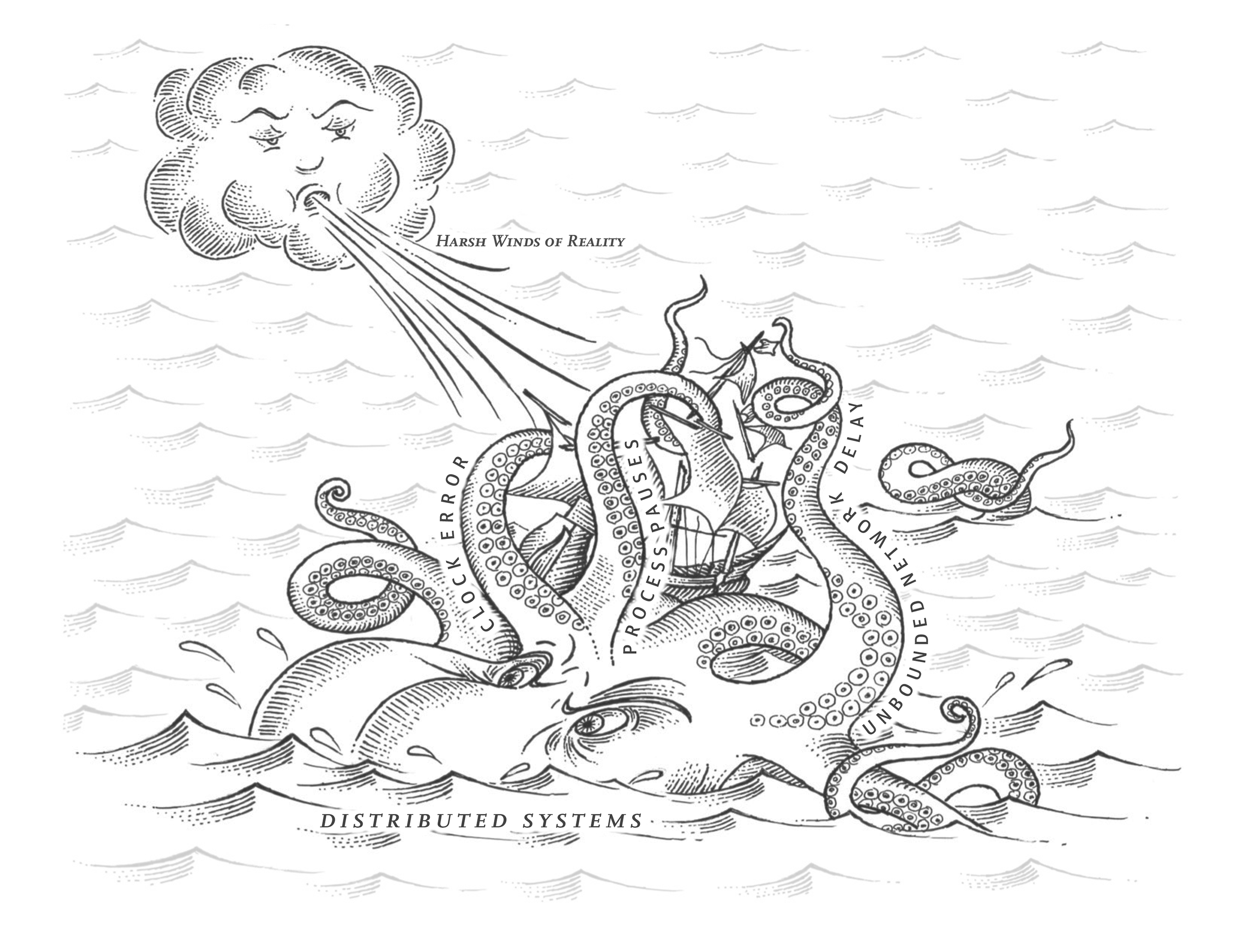
They’re funny things, Accidents. You never have them till you’re having them.

A.A. Milne, The House at Pooh Corner (1928)

As discussed in “Reliability and Fault Tolerance”, making a system reliable means ensuring that the system as a whole continues working, even when things go wrong (i.e., when there is a fault). However, anticipating all the possible faults and handling them is not that easy. As a developer, it is very tempting to focus mostly on the happy path (after all, most of the time things work fine!) and to neglect faults, since they introduce a lot of edge cases.

If you want your system to be reliable in the presence of faults you have to radically change your mindset, and focus on the things that could go wrong, even though they may be unlikely. It doesn’t matter whether there is only a one-in-a-million chance of a thing going wrong: in a large enough system, one-in-a-million events happen every day. Experienced systems operators will tell you that anything that can go wrong will go wrong.

Moreover, working with distributed systems is fundamentally different from writing software on a single computer—and the main difference is that there are lots of new and exciting ways for things to go wrong ¹ ². In this chapter, you will get a taste of the problems that arise in practice, and an understanding of the things you can and cannot rely on.

To understand what challenges we are up against, we will now turn our pessimism to the maximum and explore the things that may go wrong in a distributed system. We will look into problems with networks (“Unreliable Networks”) as well as clocks and timing issues (“Unreliable Clocks”). The consequences of all these issues are disorienting, so we’ll explore how to think about the state of a distributed system and how to reason about things that have happened (“Knowledge, Truth, and Lies”). Later, in Chapter 10, we will look at some examples of how we can achieve fault tolerance in the face of those faults.

Faults and Partial Failures

When you are writing a program on a single computer, it normally behaves in a fairly predictable way: either it works or it doesn’t. Buggy software may give the appearance that the computer is sometimes “having a bad day” (a problem that is often fixed by a reboot), but that is mostly just a consequence of badly written software.

There is no fundamental reason why software on a single computer should be flaky: when the hardware is working correctly, the same operation always produces the same result (it is deterministic). If there is a hardware problem (e.g., memory corruption or a loose connector), the consequence is usually a total system failure (e.g., kernel panic, “blue screen of death,” failure to start up). An individual computer with good software is usually either fully functional or entirely broken, but not something in between.

This is a deliberate choice in the design of computers: if an internal fault occurs, we prefer a computer to crash completely rather than returning a wrong result, because wrong results are difficult and confusing to deal with. Thus, computers hide the fuzzy physical reality on which they are implemented and present an idealized system model that operates with mathematical perfection. A CPU instruction always does the same thing; if you write some data to memory or disk, that data remains intact and doesn’t get randomly corrupted. As discussed in “Hardware and Software Faults”, this is not actually true—in reality, data does get silently corrupted and CPUs do sometimes silently return the wrong result—but it happens rarely enough that we can get away with ignoring it.

When you are writing software that runs on several computers, connected by a network, the situation is fundamentally different. In distributed systems, faults occur much more frequently, and so we can no longer ignore them—we have no choice but to confront the messy reality of the physical world. And in the physical world, a remarkably wide range of things can go wrong, as illustrated by this anecdote ³:

In my limited experience I’ve dealt with long-lived network partitions in a single data center (DC), PDU [power distribution unit] failures, switch failures, accidental power cycles of whole racks, whole-DC backbone failures, whole-DC power failures, and a hypoglycemic driver smashing his Ford pickup truck into a DC’s HVAC [heating, ventilation, and air conditioning] system. And I’m not even an ops guy.

—— Coda Hale

In a distributed system, there may well be some parts of the system that are broken in some unpredictable way, even though other parts of the system are working fine. This is known as a partial failure. The difficulty is that partial failures are nondeterministic: if you try to do anything involving multiple nodes and the network, it may sometimes work and sometimes unpredictably fail. As we shall see, you may not even know whether something succeeded or not!

This nondeterminism and possibility of partial failures is what makes distributed systems hard to work with ⁴. On the other hand, if a distributed system can tolerate partial failures, that opens up powerful possibilities: for example, it allows you to perform a rolling upgrade, rebooting one node at a time to install software updates while the system as a whole continues working uninterrupted all the time. Fault tolerance therefore allows us to make distributed systems more reliable than single-node systems: we can build a reliable system from unreliable components.

But before we can implement fault tolerance, we need to know more about the faults that we’re supposed to tolerate. It is important to consider a wide range of possible faults—even fairly unlikely ones—and to artificially create such situations in your testing environment to see what happens. In distributed systems, suspicion, pessimism, and paranoia pay off.

Unreliable Networks

As discussed in “Shared-Memory, Shared-Disk, and Shared-Nothing Architecture”, the distributed systems we focus on in this book are mostly shared-nothing systems: i.e., a bunch of machines connected by a network. The network is the only way those machines can communicate—we assume that each machine has its own memory and disk, and one machine cannot access another machine’s memory or disk (except by making requests to a service over the network). Even when storage is shared, such as with Amazon’s S3, machines communicate with shared storage services over the network.

The internet and most internal networks in datacenters (often Ethernet) are asynchronous packet networks. In this kind of network, one node can send a message (a packet) to another node, but the network gives no guarantees as to when it will arrive, or whether it will arrive at all. If you send a request and expect a response, many things could go wrong (some of which are illustrated in Figure 9-1):

Your request may have been lost (perhaps someone unplugged a network cable).
Your request may be waiting in a queue and will be delivered later (perhaps the network or the recipient is overloaded).
The remote node may have failed (perhaps it crashed or it was powered down).
The remote node may have temporarily stopped responding (perhaps it is experiencing a long garbage collection pause; see “Process Pauses”), but it will start responding again later.
The remote node may have processed your request, but the response has been lost on the network (perhaps a network switch has been misconfigured).
The remote node may have processed your request, but the response has been delayed and will be delivered later (perhaps the network or your own machine is overloaded).

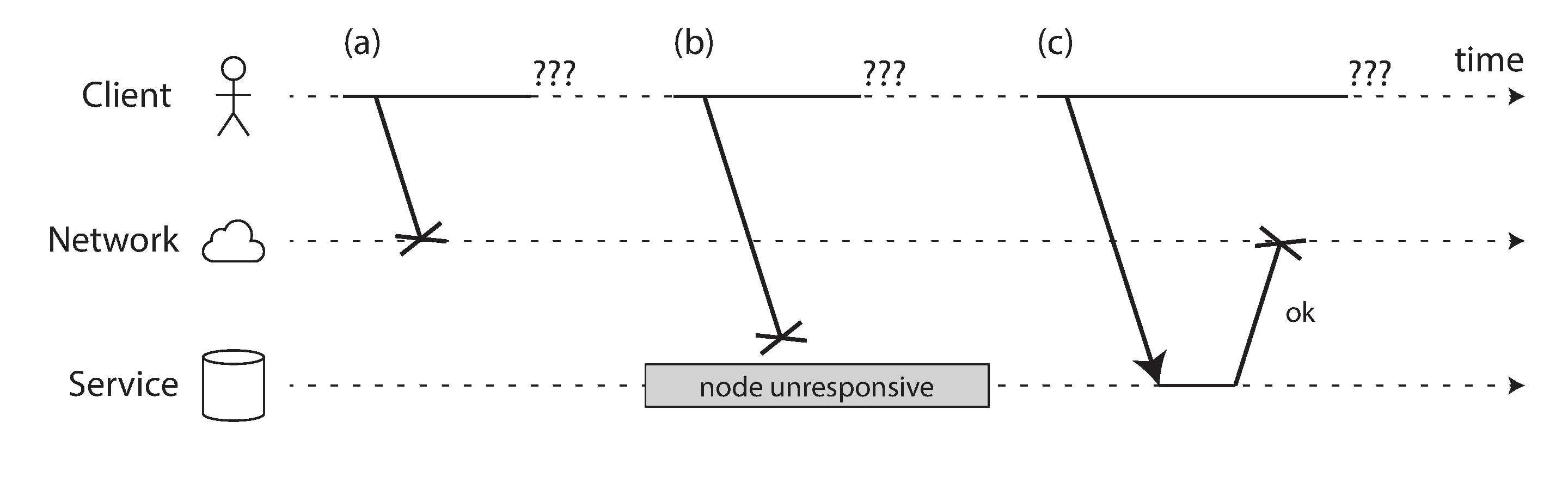
Figure 9-1 If you send a request and don't get a response, it's not possible to distinguish whether (a) the request was lost, (b) the remote node is down, or (c) the response was lost.

The sender can’t even tell whether the packet was delivered: the only option is for the recipient to send a response message, which may in turn be lost or delayed. These issues are indistinguishable in an asynchronous network: the only information you have is that you haven’t received a response yet. If you send a request to another node and don’t receive a response, it is impossible to tell why.

The usual way of handling this issue is a timeout: after some time you give up waiting and assume that the response is not going to arrive. However, when a timeout occurs, you still don’t know whether the remote node got your request or not (and if the request is still queued somewhere, it may still be delivered to the recipient, even if the sender has given up on it).

The Limitations of TCP

Network packets have a maximum size (generally a few kilobytes), but many applications need to send messages (requests, responses) that are too big to fit in one packet. These applications most often use TCP, the Transmission Control Protocol, to establish a connection that breaks up large data streams into individual packets, and puts them back together again on the receiving side.

Note

Most of what we say about TCP applies also to its more recent alternative QUIC, as well as the Stream Control Transmission Protocol (SCTP) used in WebRTC, the BitTorrent uTP protocol, and other transport protocols. For a comparison to UDP, see “TCP Versus UDP”.

TCP is often described as providing “reliable” delivery, in the sense that it detects and retransmits dropped packets, it detects reordered packets and puts them back in the correct order, and it detects packet corruption using a simple checksum. It also figures out how fast it can send data so that it is transferred as quickly as possible, but without overloading the network or the receiving node; this is known as congestion control, flow control, or backpressure ⁵.

When you “send” some data by writing it to a socket, it actually doesn’t get sent immediately, but it’s only placed in a buffer managed by your operating system. When the congestion control algorithm decides that it has capacity to send a packet, it takes the next packet-worth of data from that buffer and passes it to the network interface. The packet passes through several switches and routers, and eventually the receiving node’s operating system places the packet’s data in a receive buffer and sends an acknowledgment packet back to the sender. Only then does the receiving operating system notify the application that some more data has arrived ⁶.

So, if TCP provides “reliability”, does that mean we no longer need to worry about networks being unreliable? Unfortunately not. It decides that a packet must have been lost if no acknowledgment arrives within some timeout, but TCP can’t tell either whether it was the outbound packet or the acknowledgment that was lost. Although TCP can resend the packet, it can’t guarantee that the new packet will get through either. If the network cable is unplugged, TCP can’t plug it back in for you. Eventually, after a configurable timeout, TCP gives up and signals an error to the application.

If a TCP connection is closed with an error—perhaps because the remote node crashed, or perhaps because the network was interrupted—you unfortunately have no way of knowing how much data was actually processed by the remote node ⁶. Even if TCP acknowledged that a packet was delivered, this only means that the operating system kernel on the remote node received it, but the application may have crashed before it handled that data. If you want to be sure that a request was successful, you need a positive response from the application itself ⁷.

Nevertheless, TCP is very useful, because it provides a convenient way of sending and receiving messages that are too big to fit in one packet. Once a TCP connection is established, you can also use it to send multiple requests and responses. This is usually done by first sending a header that indicates the length of the following message in bytes, followed by the actual message. HTTP and many RPC protocols (see “Dataflow Through Services: REST and RPC”) work like this.

Network Faults in Practice

We have been building computer networks for decades—one might hope that by now we would have figured out how to make them reliable. Unfortunately, we have not yet succeeded. There are some systematic studies, and plenty of anecdotal evidence, showing that network problems can be surprisingly common, even in controlled environments like a datacenter operated by one company ⁸:

One study in a medium-sized datacenter found about 12 network faults per month, of which half disconnected a single machine, and half disconnected an entire rack ⁹.
Another study measured the failure rates of components like top-of-rack switches, aggregation switches, and load balancers ¹⁰. It found that adding redundant networking gear doesn’t reduce faults as much as you might hope, since it doesn’t guard against human error (e.g., misconfigured switches), which is a major cause of outages.
Interruptions of wide-area fiber links have been blamed on cows ¹¹, beavers ¹², and sharks ¹³ (though shark bites have become rarer due to better shielding of submarine cables ¹⁴). Humans are also at fault, be it due to accidental misconfiguration ¹⁵, scavenging ¹⁶, or sabotage ¹⁷.
Across different cloud regions, round-trip times of up to several minutes have been observed at high percentiles ¹⁸. Even within a single datacenter, packet delay of more than a minute can occur during a network topology reconfiguration, triggered by a problem during a software upgrade for a switch ¹⁹. Thus, we have to assume that messages might be delayed arbitrarily.
Sometimes communications are partially interrupted, depending on who you’re talking to: for example, A and B can communicate, B and C can communicate, but A and C cannot ²⁰ ²¹. Other surprising faults include a network interface that sometimes drops all inbound packets but sends outbound packets successfully ²²: just because a network link works in one direction doesn’t guarantee it’s also working in the opposite direction.
Even a brief network interruption can have repercussions that last for much longer than the original issue ⁸ ²⁰ ²³.

NETWORK PARTITIONS

When one part of the network is cut off from the rest due to a network fault, that is sometimes called a network partition or netsplit, but it is not fundamentally different from other kinds of network interruption. Network partitions are not related to sharding of a storage system, which is sometimes also called partitioning (see Chapter 7).

Even if network faults are rare in your environment, the fact that faults can occur means that your software needs to be able to handle them. Whenever any communication happens over a network, it may fail—there is no way around it.

If the error handling of network faults is not defined and tested, arbitrarily bad things could happen: for example, the cluster could become deadlocked and permanently unable to serve requests, even when the network recovers ²⁴, or it could even delete all of your data ²⁵. If software is put in an unanticipated situation, it may do arbitrary unexpected things.

Handling network faults doesn’t necessarily mean tolerating them: if your network is normally fairly reliable, a valid approach may be to simply show an error message to users while your network is experiencing problems. However, you do need to know how your software reacts to network problems and ensure that the system can recover from them. It may make sense to deliberately trigger network problems and test the system’s response (this is known as fault injection; see “Fault injection”).

Detecting Faults

Many systems need to automatically detect faulty nodes. For example:

A load balancer needs to stop sending requests to a node that is dead (i.e., take it out of rotation).
In a distributed database with single-leader replication, if the leader fails, one of the followers needs to be promoted to be the new leader (see “Handling Node Outages”).

Unfortunately, the uncertainty about the network makes it difficult to tell whether a node is working or not. In some specific circumstances you might get some feedback to explicitly tell you that something is not working:

If you can reach the machine on which the node should be running, but no process is listening on the destination port (e.g., because the process crashed), the operating system will helpfully close or refuse TCP connections by sending a RST or FIN packet in reply.
If a node process crashed (or was killed by an administrator) but the node’s operating system is still running, a script can notify other nodes about the crash so that another node can take over quickly without having to wait for a timeout to expire. For example, HBase does this ²⁶.
If you have access to the management interface of the network switches in your datacenter, you can query them to detect link failures at a hardware level (e.g., if the remote machine is powered down). This option is ruled out if you’re connecting via the internet, or if you’re in a shared datacenter with no access to the switches themselves, or if you can’t reach the management interface due to a network problem.
If a router is sure that the IP address you’re trying to connect to is unreachable, it may reply to you with an ICMP Destination Unreachable packet. However, the router doesn’t have a magic failure detection capability either—it is subject to the same limitations as other participants of the network.

Rapid feedback about a remote node being down is useful, but you can’t count on it. If something has gone wrong, you may get an error response at some level of the stack, but in general you have to assume that you will get no response at all. You can retry a few times, wait for a timeout to elapse, and eventually declare the node dead if you don’t hear back within the timeout.

Timeouts and Unbounded Delays

If a timeout is the only sure way of detecting a fault, then how long should the timeout be? There is unfortunately no simple answer.

A long timeout means a long wait until a node is declared dead (and during this time, users may have to wait or see error messages). A short timeout detects faults faster, but carries a higher risk of incorrectly declaring a node dead when in fact it has only suffered a temporary slowdown (e.g., due to a load spike on the node or the network).

Prematurely declaring a node dead is problematic: if the node is actually alive and in the middle of performing some action (for example, sending an email), and another node takes over, the action may end up being performed twice. We will discuss this issue in more detail in “Knowledge, Truth, and Lies”, Chapter 10, and “The End-to-End Argument for Databases”.

When a node is declared dead, its responsibilities need to be transferred to other nodes, which places additional load on other nodes and the network. If the system is already struggling with high load, declaring nodes dead prematurely can make the problem worse. In particular, it could happen that the node actually wasn’t dead but only slow to respond due to overload; transferring its load to other nodes can cause a cascading failure (in the extreme case, all nodes declare each other dead, and everything stops working—see “When an overloaded system won’t recover”).

Imagine a fictitious system with a network that guaranteed a maximum delay for packets—every packet is either delivered within some time d, or it is lost, but delivery never takes longer than d. Furthermore, assume that you can guarantee that a non-failed node always handles a request within some time r. In this case, you could guarantee that every successful request receives a response within time 2d + r—and if you don’t receive a response within that time, you know that either the network or the remote node is not working. If this was true, 2d + r would be a reasonable timeout to use.

Unfortunately, most systems we work with have neither of those guarantees: asynchronous networks have unbounded delays (that is, they try to deliver packets as quickly as possible, but there is no upper limit on the time it may take for a packet to arrive), and most server implementations cannot guarantee that they can handle requests within some maximum time (see “Response time guarantees”). For failure detection, it’s not sufficient for the system to be fast most of the time: if your timeout is low, it only takes a transient spike in round-trip times to throw the system off-balance.

Network congestion and queueing

When driving a car, travel times on road networks often vary most due to traffic congestion. Similarly, the variability of packet delays on computer networks is most often due to queueing ²⁷:

If several different nodes simultaneously try to send packets to the same destination, the network switch must queue them up and feed them into the destination network link one by one (as illustrated in Figure 9-2). On a busy network link, a packet may have to wait a while until it can get a slot (this is called network congestion). If there is so much incoming data that the switch queue fills up, the packet is dropped, so it needs to be resent—even though the network is functioning fine.
When a packet reaches the destination machine, if all CPU cores are currently busy, the incoming request from the network is queued by the operating system until the application is ready to handle it. Depending on the load on the machine, this may take an arbitrary length of time ²⁸.
In virtualized environments, a running operating system is often paused for tens of milliseconds while another virtual machine uses a CPU core. During this time, the VM cannot consume any data from the network, so the incoming data is queued (buffered) by the virtual machine monitor ²⁹, further increasing the variability of network delays.
As mentioned earlier, in order to avoid overloading the network, TCP limits the rate at which it sends data. This means additional queueing at the sender before the data even enters the network.

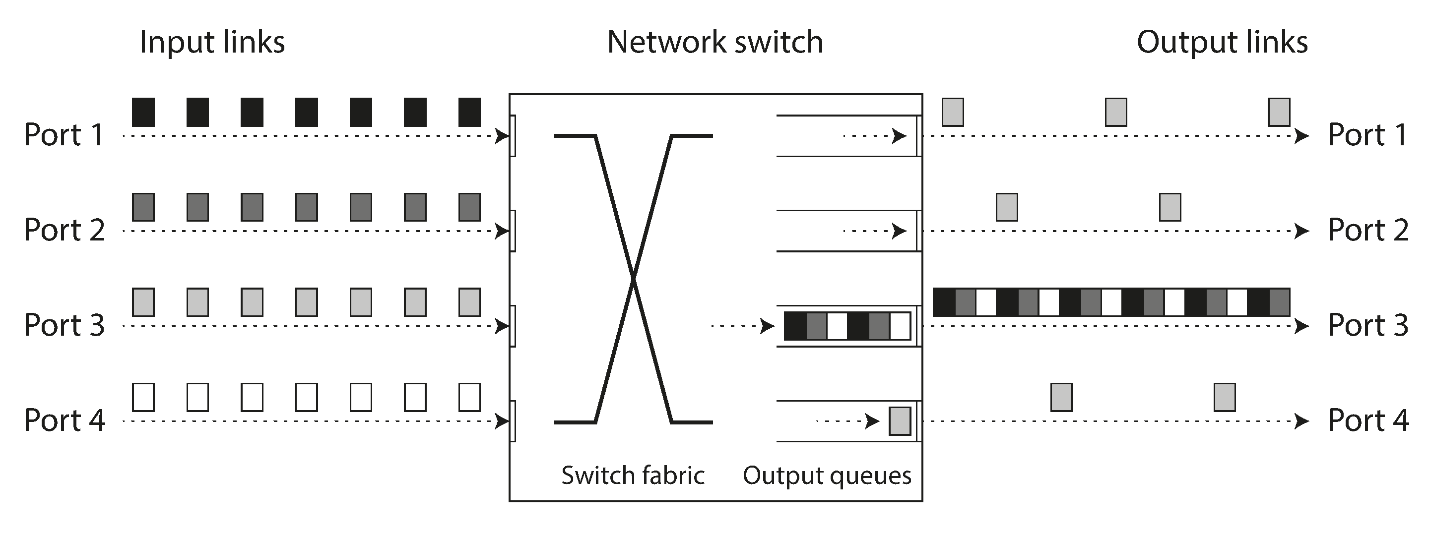
Figure 9-2 If several machines send network traffic to the same destination, its switch queue can fill up. Here, ports 1, 2, and 4 are all trying to send packets to port 3.

Moreover, when TCP detects and automatically retransmits a lost packet, although the application does not see the packet loss directly, it does see the resulting delay (waiting for the timeout to expire, and then waiting for the retransmitted packet to be acknowledged).

TCP VERSUS UDP

Some latency-sensitive applications, such as videoconferencing and Voice over IP (VoIP), use UDP rather than TCP. It’s a trade-off between reliability and variability of delays: as UDP does not perform flow control and does not retransmit lost packets, it avoids some of the reasons for variable network delays (although it is still susceptible to switch queues and scheduling delays).

UDP is a good choice in situations where delayed data is worthless. For example, in a VoIP phone call, there probably isn’t enough time to retransmit a lost packet before its data is due to be played over the loudspeakers. In this case, there’s no point in retransmitting the packet—the application must instead fill the missing packet’s time slot with silence (causing a brief interruption in the sound) and move on in the stream. The retry happens at the human layer instead. (“Could you repeat that please? The sound just cut out for a moment.”)

All of these factors contribute to the variability of network delays. Queueing delays have an especially wide range when a system is close to its maximum capacity: a system with plenty of spare capacity can easily drain queues, whereas in a highly utilized system, long queues can build up very quickly.

In public clouds and multitenant datacenters, resources are shared among many customers: the network links and switches, and even each machine’s network interface and CPUs (when running on virtual machines), are shared. Processing large amounts of data can use the entire capacity of network links (saturate them). As you have no control over or insight into other customers’ usage of the shared resources, network delays can be highly variable if someone near you (a noisy neighbor) is using a lot of resources ³⁰ ³¹.

In such environments, you can only choose timeouts experimentally: measure the distribution of network round-trip times over an extended period, and over many machines, to determine the expected variability of delays. Then, taking into account your application’s characteristics, you can determine an appropriate trade-off between failure detection delay and risk of premature timeouts.

Even better, rather than using configured constant timeouts, systems can continually measure response times and their variability (jitter), and automatically adjust timeouts according to the observed response time distribution. The Phi Accrual failure detector ³², which is used for example in Akka and Cassandra ³³ is one way of doing this. TCP retransmission timeouts also work similarly ⁵.

Synchronous Versus Asynchronous Networks

Distributed systems would be a lot simpler if we could rely on the network to deliver packets with some fixed maximum delay, and not to drop packets. Why can’t we solve this at the hardware level and make the network reliable so that the software doesn’t need to worry about it?

To answer this question, it’s interesting to compare datacenter networks to the traditional fixed-line telephone network (non-cellular, non-VoIP), which is extremely reliable: delayed audio frames and dropped calls are very rare. A phone call requires a constantly low end-to-end latency and enough bandwidth to transfer the audio samples of your voice. Wouldn’t it be nice to have similar reliability and predictability in computer networks?

When you make a call over the telephone network, it establishes a circuit: a fixed, guaranteed amount of bandwidth is allocated for the call, along the entire route between the two callers. This circuit remains in place until the call ends ³⁴. For example, an ISDN network runs at a fixed rate of 4,000 frames per second. When a call is established, it is allocated 16 bits of space within each frame (in each direction). Thus, for the duration of the call, each side is guaranteed to be able to send exactly 16 bits of audio data every 250 microseconds ³⁵.

This kind of network is synchronous: even as data passes through several routers, it does not suffer from queueing, because the 16 bits of space for the call have already been reserved in the next hop of the network. And because there is no queueing, the maximum end-to-end latency of the network is fixed. We call this a bounded delay.

Can we not simply make network delays predictable?

Note that a circuit in a telephone network is very different from a TCP connection: a circuit is a fixed amount of reserved bandwidth which nobody else can use while the circuit is established, whereas the packets of a TCP connection opportunistically use whatever network bandwidth is available. You can give TCP a variable-sized block of data (e.g., an email or a web page), and it will try to transfer it in the shortest time possible. While a TCP connection is idle, it doesn’t use any bandwidth (except perhaps for an occasional keepalive packet).

If datacenter networks and the internet were circuit-switched networks, it would be possible to establish a guaranteed maximum round-trip time when a circuit was set up. However, they are not: Ethernet and IP are packet-switched protocols, which suffer from queueing and thus unbounded delays in the network. These protocols do not have the concept of a circuit.

Why do datacenter networks and the internet use packet switching? The answer is that they are optimized for bursty traffic. A circuit is good for an audio or video call, which needs to transfer a fairly constant number of bits per second for the duration of the call. On the other hand, requesting a web page, sending an email, or transferring a file doesn’t have any particular bandwidth requirement—we just want it to complete as quickly as possible.

If you wanted to transfer a file over a circuit, you would have to guess a bandwidth allocation. If you guess too low, the transfer is unnecessarily slow, leaving network capacity unused. If you guess too high, the circuit cannot be set up (because the network cannot allow a circuit to be created if its bandwidth allocation cannot be guaranteed). Thus, using circuits for bursty data transfers wastes network capacity and makes transfers unnecessarily slow. By contrast, TCP dynamically adapts the rate of data transfer to the available network capacity.

There have been some attempts to build hybrid networks that support both circuit switching and packet switching. Asynchronous Transfer Mode (ATM) was a competitor to Ethernet in the 1980s, but it didn’t gain much adoption outside of telephone network core switches. InfiniBand has some similarities ³⁶: it implements end-to-end flow control at the link layer, which reduces the need for queueing in the network, although it can still suffer from delays due to link congestion ³⁷. With careful use of quality of service (QoS, prioritization and scheduling of packets) and admission control (rate-limiting senders), it is possible to emulate circuit switching on packet networks, or provide statistically bounded delay ²⁷ ³⁴. New network algorithms like Low Latency, Low Loss, and Scalable Throughput (L4S) attempt to mitigate some of the queuing and congestion control problems both at the client and router level. Linux’s traffic controller (TC) also allows applications to reprioritize packets for QoS purposes.

LATENCY AND RESOURCE UTILIZATION

More generally, you can think of variable delays as a consequence of dynamic resource partitioning.

Say you have a wire between two telephone switches that can carry up to 10,000 simultaneous calls. Each circuit that is switched over this wire occupies one of those call slots. Thus, you can think of the wire as a resource that can be shared by up to 10,000 simultaneous users. The resource is divided up in a static way: even if you’re the only call on the wire right now, and all other 9,999 slots are unused, your circuit is still allocated the same fixed amount of bandwidth as when the wire is fully utilized.

By contrast, the internet shares network bandwidth dynamically. Senders push and jostle with each other to get their packets over the wire as quickly as possible, and the network switches decide which packet to send (i.e., the bandwidth allocation) from one moment to the next. This approach has the downside of queueing, but the advantage is that it maximizes utilization of the wire. The wire has a fixed cost, so if you utilize it better, each byte you send over the wire is cheaper.

A similar situation arises with CPUs: if you share each CPU core dynamically between several threads, one thread sometimes has to wait in the operating system’s run queue while another thread is running, so a thread can be paused for varying lengths of time ³⁸. However, this utilizes the hardware better than if you allocated a static number of CPU cycles to each thread (see “Response time guarantees”). Better hardware utilization is also why cloud platforms run several virtual machines from different customers on the same physical machine.

Latency guarantees are achievable in certain environments, if resources are statically partitioned (e.g., dedicated hardware and exclusive bandwidth allocations). However, it comes at the cost of reduced utilization—in other words, it is more expensive. On the other hand, multitenancy with dynamic resource partitioning provides better utilization, so it is cheaper, but it has the downside of variable delays.

Variable delays in networks are not a law of nature, but simply the result of a cost/benefit trade-off.

However, such quality of service is currently not enabled in multitenant datacenters and public clouds, or when communicating via the internet. Currently deployed technology does not allow us to make any guarantees about delays or reliability of the network: we have to assume that network congestion, queueing, and unbounded delays will happen. Consequently, there’s no “correct” value for timeouts—they need to be determined experimentally.

Peering agreements between internet service providers and the establishment of routes through the Border Gateway Protocol (BGP), bear closer resemblance to circuit switching than IP itself. At this level, it is possible to buy dedicated bandwidth. However, internet routing operates at the level of networks, not individual connections between hosts, and at a much longer timescale.

Unreliable Clocks

Clocks and time are important. Applications depend on clocks in various ways to answer questions like the following:

Has this request timed out yet?
What’s the 99th percentile response time of this service?
How many queries per second did this service handle on average in the last five minutes?
How long did the user spend on our site?
When was this article published?
At what date and time should the reminder email be sent?
When does this cache entry expire?
What is the timestamp on this error message in the log file?

Examples 1–4 measure durations (e.g., the time interval between a request being sent and a response being received), whereas examples 5–8 describe points in time (events that occur on a particular date, at a particular time).

In a distributed system, time is a tricky business, because communication is not instantaneous: it takes time for a message to travel across the network from one machine to another. The time when a message is received is always later than the time when it is sent, but due to variable delays in the network, we don’t know how much later. This fact sometimes makes it difficult to determine the order in which things happened when multiple machines are involved.

Moreover, each machine on the network has its own clock, which is an actual hardware device: usually a quartz crystal oscillator. These devices are not perfectly accurate, so each machine has its own notion of time, which may be slightly faster or slower than on other machines. It is possible to synchronize clocks to some degree: the most commonly used mechanism is the Network Time Protocol (NTP), which allows the computer clock to be adjusted according to the time reported by a group of servers ³⁹. The servers in turn get their time from a more accurate time source, such as a GPS receiver.

Monotonic Versus Time-of-Day Clocks

Modern computers have at least two different kinds of clocks: a time-of-day clock and a monotonic clock. Although they both measure time, it is important to distinguish the two, since they serve different purposes.

Time-of-day clocks

A time-of-day clock does what you intuitively expect of a clock: it returns the current date and time according to some calendar (also known as wall-clock time). For example, clock_gettime(CLOCK_REALTIME) on Linux and System.currentTimeMillis() in Java return the number of seconds (or milliseconds) since the epoch: midnight UTC on January 1, 1970, according to the Gregorian calendar, not counting leap seconds. Some systems use other dates as their reference point. (Although the Linux clock is called real-time, it has nothing to do with real-time operating systems, as discussed in “Response time guarantees”.)

Time-of-day clocks are usually synchronized with NTP, which means that a timestamp from one machine (ideally) means the same as a timestamp on another machine. However, time-of-day clocks also have various oddities, as described in the next section. In particular, if the local clock is too far ahead of the NTP server, it may be forcibly reset and appear to jump back to a previous point in time. These jumps, as well as similar jumps caused by leap seconds, make time-of-day clocks unsuitable for measuring elapsed time ⁴⁰.

Time-of-day clocks can experience jumps due to the start and end of Daylight Saving Time (DST); these can be avoided by always using UTC as time zone, which does not have DST. Time-of-day clocks have also historically had quite a coarse-grained resolution, e.g., moving forward in steps of 10 ms on older Windows systems ⁴¹. On recent systems, this is less of a problem.

Monotonic clocks

A monotonic clock is suitable for measuring a duration (time interval), such as a timeout or a service’s response time: clock_gettime(CLOCK_MONOTONIC) or clock_gettime(CLOCK_BOOTTIME) on Linux ⁴² and System.nanoTime() in Java are monotonic clocks, for example. The name comes from the fact that they are guaranteed to always move forward (whereas a time-of-day clock may jump back in time).

You can check the value of the monotonic clock at one point in time, do something, and then check the clock again at a later time. The difference between the two values tells you how much time elapsed between the two checks — more like a stopwatch than a wall clock. However, the absolute value of the clock is meaningless: it might be the number of nanoseconds since the computer was booted up, or something similarly arbitrary. In particular, it makes no sense to compare monotonic clock values from two different computers, because they don’t mean the same thing.

On a server with multiple CPU sockets, there may be a separate timer per CPU, which is not necessarily synchronized with other CPUs ⁴³. Operating systems compensate for any discrepancy and try to present a monotonic view of the clock to application threads, even as they are scheduled across different CPUs. However, it is wise to take this guarantee of monotonicity with a pinch of salt ⁴⁴.

NTP may adjust the frequency at which the monotonic clock moves forward (this is known as slewing the clock) if it detects that the computer’s local quartz is moving faster or slower than the NTP server. By default, NTP allows the clock rate to be speeded up or slowed down by up to 0.05%, but NTP cannot cause the monotonic clock to jump forward or backward. The resolution of monotonic clocks is usually quite good: on most systems they can measure time intervals in microseconds or less.

In a distributed system, using a monotonic clock for measuring elapsed time (e.g., timeouts) is usually fine, because it doesn’t assume any synchronization between different nodes’ clocks and is not sensitive to slight inaccuracies of measurement.

Clock Synchronization and Accuracy

Monotonic clocks don’t need synchronization, but time-of-day clocks need to be set according to an NTP server or other external time source in order to be useful. Unfortunately, our methods for getting a clock to tell the correct time aren’t nearly as reliable or accurate as you might hope—hardware clocks and NTP can be fickle beasts. To give just a few examples:

The quartz clock in a computer is not very accurate: it drifts (runs faster or slower than it should). Clock drift varies depending on the temperature of the machine. Google assumes a clock drift of up to 200 ppm (parts per million) for its servers ⁴⁵, which is equivalent to 6 ms drift for a clock that is resynchronized with a server every 30 seconds, or 17 seconds drift for a clock that is resynchronized once a day. This drift limits the best possible accuracy you can achieve, even if everything is working correctly.
If a computer’s clock differs too much from an NTP server, it may refuse to synchronize, or the local clock will be forcibly reset ³⁹. Any applications observing the time before and after this reset may see time go backward or suddenly jump forward.
If a node is accidentally firewalled off from NTP servers, the misconfiguration may go unnoticed for some time, during which the drift may add up to large discrepancies between different nodes’ clocks. Anecdotal evidence suggests that this does happen in practice.
NTP synchronization can only be as good as the network delay, so there is a limit to its accuracy when you’re on a congested network with variable packet delays. One experiment showed that a minimum error of 35 ms is achievable when synchronizing over the internet ⁴⁶, though occasional spikes in network delay lead to errors of around a second. Depending on the configuration, large network delays can cause the NTP client to give up entirely.
Some NTP servers are wrong or misconfigured, reporting time that is off by hours ⁴⁷ ⁴⁸. NTP clients mitigate such errors by querying several servers and ignoring outliers. Nevertheless, it’s somewhat worrying to bet the correctness of your systems on the time that you were told by a stranger on the internet.
Leap seconds result in a minute that is 59 seconds or 61 seconds long, which messes up timing assumptions in systems that are not designed with leap seconds in mind ⁴⁹. The fact that leap seconds have crashed many large systems ⁴⁰ ⁵⁰ shows how easy it is for incorrect assumptions about clocks to sneak into a system. The best way of handling leap seconds may be to make NTP servers “lie,” by performing the leap second adjustment gradually over the course of a day (this is known as smearing) ⁵¹ ⁵², although actual NTP server behavior varies in practice ⁵³. Leap seconds will no longer be used from 2035 onwards, so this problem will fortunately go away.
In virtual machines, the hardware clock is virtualized, which raises additional challenges for applications that need accurate timekeeping ⁵⁴. When a CPU core is shared between virtual machines, each VM is paused for tens of milliseconds while another VM is running. From an application’s point of view, this pause manifests itself as the clock suddenly jumping forward ²⁹. If a VM pauses for several seconds, the clock may then be several seconds behind the actual time, but NTP may continue to report that the clock is almost perfectly in sync ⁵⁵.
If you run software on devices that you don’t fully control (e.g., mobile or embedded devices), you probably cannot trust the device’s hardware clock at all. Some users deliberately set their hardware clock to an incorrect date and time, for example to cheat in games ⁵⁶. As a result, the clock might be set to a time wildly in the past or the future.

It is possible to achieve very good clock accuracy if you care about it sufficiently to invest significant resources. For example, the MiFID II European regulation for financial institutions requires all high-frequency trading funds to synchronize their clocks to within 100 microseconds of UTC, in order to help debug market anomalies such as “flash crashes” and to help detect market manipulation ⁵⁷.

Such accuracy can be achieved with some special hardware (GPS receivers and/or atomic clocks), the Precision Time Protocol (PTP) and careful deployment and monitoring ⁵⁸ ⁵⁹. Relying on GPS alone can be risky because GPS signals can easily be jammed. In some locations this happens frequently, e.g. close to military facilities ⁶⁰. Some cloud providers have begun offering high-accuracy clock synchronization for their virtual machines ⁶¹. However, clock synchronization still requires a lot of care. If your NTP daemon is misconfigured, or a firewall is blocking NTP traffic, the clock error due to drift can quickly become large.

Relying on Synchronized Clocks

The problem with clocks is that while they seem simple and easy to use, they have a surprising number of pitfalls: a day may not have exactly 86,400 seconds, time-of-day clocks may move backward in time, and the time according to one node’s clock may be quite different from another node’s clock.

Earlier in this chapter we discussed networks dropping and arbitrarily delaying packets. Even though networks are well behaved most of the time, software must be designed on the assumption that the network will occasionally be faulty, and the software must handle such faults gracefully. The same is true with clocks: although they work quite well most of the time, robust software needs to be prepared to deal with incorrect clocks.

Part of the problem is that incorrect clocks easily go unnoticed. If a machine’s CPU is defective or its network is misconfigured, it most likely won’t work at all, so it will quickly be noticed and fixed. On the other hand, if its quartz clock is defective or its NTP client is misconfigured, most things will seem to work fine, even though its clock gradually drifts further and further away from reality. If some piece of software is relying on an accurately synchronized clock, the result is more likely to be silent and subtle data loss than a dramatic crash ⁶² ⁶³.

Thus, if you use software that requires synchronized clocks, it is essential that you also carefully monitor the clock offsets between all the machines. Any node whose clock drifts too far from the others should be declared dead and removed from the cluster. Such monitoring ensures that you notice the broken clocks before they can cause too much damage.

Timestamps for ordering events

Let’s consider one particular situation in which it is tempting, but dangerous, to rely on clocks: ordering of events across multiple nodes ⁶⁴. For example, if two clients write to a distributed database, who got there first? Which write is the more recent one?

Figure 9-3 illustrates a dangerous use of time-of-day clocks in a database with multi-leader replication (the example is similar to Figure 6-8). Client A writes x = 1 on node 1; the write is replicated to node 3; client B increments x on node 3 (we now have x = 2); and finally, both writes are replicated to node 2.

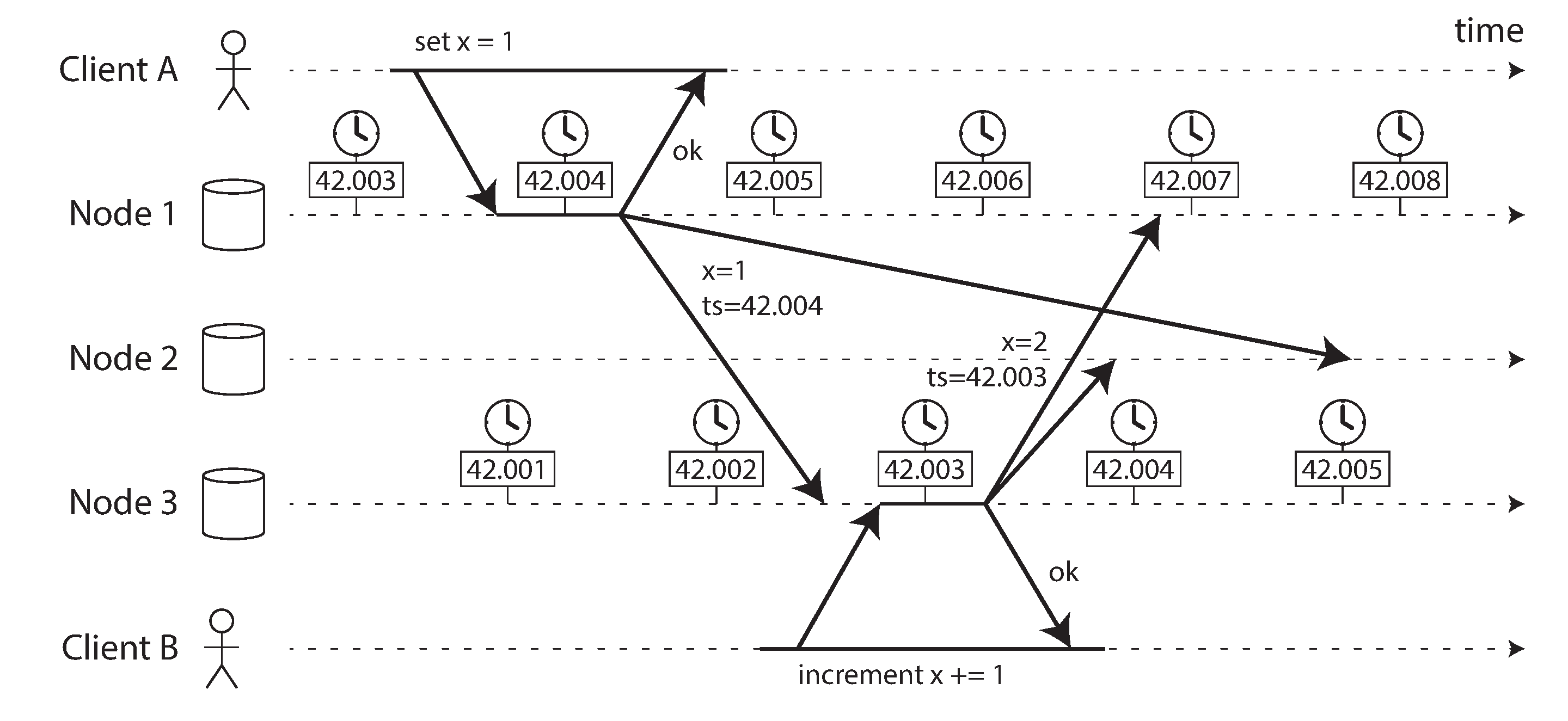
Figure 9-3 The write by client B is causally later than the write by client A, but B's write has an earlier timestamp.

In Figure 9-3, when a write is replicated to other nodes, it is tagged with a timestamp according to the time-of-day clock on the node where the write originated. The clock synchronization is very good in this example: the skew between node 1 and node 3 is less than 3 ms, which is probably better than you can expect in practice.

Since the increment builds upon the earlier write of x = 1, we might expect that the write of x = 2 should have the greater timestamp of the two. Unfortunately, that is not what happens in Figure 9-3: the write x = 1 has a timestamp of 42.004 seconds, but the write x = 2 has a timestamp of 42.003 seconds.

As discussed in “Last write wins (discarding concurrent writes)”, one way of resolving conflicts between concurrently written values on different nodes is last write wins (LWW), which means keeping the write with the greatest timestamp for a given key and discarding all writes with older timestamps. In the example of Figure 9-3, when node 2 receives these two events, it will incorrectly conclude that x = 1 is the more recent value and drop the write x = 2, so the increment is lost.

This problem can be prevented by ensuring that when a value is overwritten, the new value always has a higher timestamp than the overwritten value, even if that timestamp is ahead of the writer’s local clock. However, that incurs the cost of an additional read to find the greatest existing timestamp. Some systems, including Cassandra and ScyllaDB, want to write to all replicas in a single round trip, and therefore they simply use the client clock’s timestamp along with a last write wins policy ⁶². This approach has some serious problems:

Database writes can mysteriously disappear: a node with a lagging clock is unable to overwrite values previously written by a node with a fast clock until the clock skew between the nodes has elapsed ⁶³ ⁶⁵. This scenario can cause arbitrary amounts of data to be silently dropped without any error being reported to the application.
LWW cannot distinguish between writes that occurred sequentially in quick succession (in Figure 9-3, client B’s increment definitely occurs after client A’s write) and writes that were truly concurrent (neither writer was aware of the other). Additional causality tracking mechanisms, such as version vectors, are needed in order to prevent violations of causality (see “Detecting Concurrent Writes”).
It is possible for two nodes to independently generate writes with the same timestamp, especially when the clock only has millisecond resolution. An additional tiebreaker value (which can simply be a large random number) is required to resolve such conflicts, but this approach can also lead to violations of causality ⁶².

Thus, even though it is tempting to resolve conflicts by keeping the most “recent” value and discarding others, it’s important to be aware that the definition of “recent” depends on a local time-of-day clock, which may well be incorrect. Even with tightly NTP-synchronized clocks, you could send a packet at timestamp 100 ms (according to the sender’s clock) and have it arrive at timestamp 99 ms (according to the recipient’s clock)—so it appears as though the packet arrived before it was sent, which is impossible.

Could NTP synchronization be made accurate enough that such incorrect orderings cannot occur? Probably not, because NTP’s synchronization accuracy is itself limited by the network round-trip time, in addition to other sources of error such as quartz drift. To guarantee a correct ordering, you would need the clock error to be significantly lower than the network delay, which is not possible.

So-called logical clocks ⁶⁶, which are based on incrementing counters rather than an oscillating quartz crystal, are a safer alternative for ordering events (see “Detecting Concurrent Writes”). Logical clocks do not measure the time of day or the number of seconds elapsed, only the relative ordering of events (whether one event happened before or after another). In contrast, time-of-day and monotonic clocks, which measure actual elapsed time, are also known as physical clocks. We’ll look at logical clocks in more detail in “ID Generators and Logical Clocks”.

Clock readings with a confidence interval

You may be able to read a machine’s time-of-day clock with microsecond or even nanosecond resolution. But even if you can get such a fine-grained measurement, that doesn’t mean the value is actually accurate to such precision. In fact, it most likely is not—as mentioned previously, the drift in an imprecise quartz clock can easily be several milliseconds, even if you synchronize with an NTP server on the local network every minute. With an NTP server on the public internet, the best possible accuracy is probably to the tens of milliseconds, and the error may easily spike to over 100 ms when there is network congestion.

Thus, it doesn’t make sense to think of a clock reading as a point in time—it is more like a range of times, within a confidence interval: for example, a system may be 95% confident that the time now is between 10.3 and 10.5 seconds past the minute, but it doesn’t know any more precisely than that ⁶⁷. If we only know the time +/– 100 ms, the microsecond digits in the timestamp are essentially meaningless.

The uncertainty bound can be calculated based on your time source. If you have a GPS receiver or atomic clock directly attached to your computer, the expected error range is determined by the device and, in the case of GPS, by the quality of the signal from the satellites. If you’re getting the time from a server, the uncertainty is based on the expected quartz drift since your last sync with the server, plus the NTP server’s uncertainty, plus the network round-trip time to the server (to a first approximation, and assuming you trust the server).

Unfortunately, most systems don’t expose this uncertainty: for example, when you call clock_gettime(), the return value doesn’t tell you the expected error of the timestamp, so you don’t know if its confidence interval is five milliseconds or five years.

There are exceptions: the TrueTime API in Google’s Spanner ⁴⁵ and Amazon’s ClockBound explicitly report the confidence interval on the local clock. When you ask it for the current time, you get back two values: [earliest, latest], which are the earliest possible and the latest possible timestamp. Based on its uncertainty calculations, the clock knows that the actual current time is somewhere within that interval. The width of the interval depends, among other things, on how long it has been since the local quartz clock was last synchronized with a more accurate clock source.

Synchronized clocks for global snapshots

In “Snapshot Isolation and Repeatable Read” we discussed multi-version concurrency control (MVCC), which is a very useful feature in databases that need to support both small, fast read-write transactions and large, long-running read-only transactions (e.g., for backups or analytics). It allows read-only transactions to see a snapshot of the database, a consistent state at a particular point in time, without locking and interfering with read-write transactions.

Generally, MVCC requires a monotonically increasing transaction ID. If a write happened later than the snapshot (i.e., the write has a greater transaction ID than the snapshot), that write is invisible to the snapshot transaction. On a single-node database, a simple counter is sufficient for generating transaction IDs.

However, when a database is distributed across many machines, potentially in multiple datacenters, a global, monotonically increasing transaction ID (across all shards) is difficult to generate, because it requires coordination. The transaction ID must reflect causality: if transaction B reads or overwrites a value that was previously written by transaction A, then B must have a higher transaction ID than A—otherwise, the snapshot would not be consistent. With lots of small, rapid transactions, creating transaction IDs in a distributed system becomes an untenable bottleneck. (We will discuss such ID generators in “ID Generators and Logical Clocks”.)

Can we use the timestamps from synchronized time-of-day clocks as transaction IDs? If we could get the synchronization good enough, they would have the right properties: later transactions have a higher timestamp. The problem, of course, is the uncertainty about clock accuracy.

Spanner implements snapshot isolation across datacenters in this way ⁶⁸ ⁶⁹. It uses the clock’s confidence interval as reported by the TrueTime API, and is based on the following observation: if you have two confidence intervals, each consisting of an earliest and latest possible timestamp (A = [Aearliest, Alatest] and B = [Bearliest, Blatest]), and those two intervals do not overlap (i.e., Aearliest < Alatest < Bearliest < Blatest), then B definitely happened after A—there can be no doubt. Only if the intervals overlap are we unsure in which order A and B happened.

In order to ensure that transaction timestamps reflect causality, Spanner deliberately waits for the length of the confidence interval before committing a read-write transaction. By doing so, it ensures that any transaction that may read the data is at a sufficiently later time, so their confidence intervals do not overlap. In order to keep the wait time as short as possible, Spanner needs to keep the clock uncertainty as small as possible; for this purpose, Google deploys a GPS receiver or atomic clock in each datacenter, allowing clocks to be synchronized to within about 7 ms ⁴⁵.

The atomic clocks and GPS receivers are not strictly necessary in Spanner: the important thing is to have a confidence interval, and the accurate clock sources only help keep that interval small. Other systems are beginning to adopt similar approaches: for example, YugabyteDB can leverage ClockBound when running on AWS ⁷⁰, and several other systems now also rely on clock synchronization to various degrees ⁷¹ ⁷².

Process Pauses

Let’s consider another example of dangerous clock use in a distributed system. Say you have a database with a single leader per shard. Only the leader is allowed to accept writes. How does a node know that it is still leader (that it hasn’t been declared dead by the others), and that it may safely accept writes?

One option is for the leader to obtain a lease from the other nodes, which is similar to a lock with a timeout ⁷³. Only one node can hold the lease at any one time—thus, when a node obtains a lease, it knows that it is the leader for some amount of time, until the lease expires. In order to remain leader, the node must periodically renew the lease before it expires. If the node fails, it stops renewing the lease, so another node can take over when it expires.

You can imagine the request-handling loop looking something like this:

while (true) {
    request = getIncomingRequest();

    // Ensure that the lease always has at least 10 seconds remaining
    if (lease.expiryTimeMillis - System.currentTimeMillis() < 10000) {
        lease = lease.renew();
    }

    if (lease.isValid()) {
        process(request);
    }
}

What’s wrong with this code? Firstly, it’s relying on synchronized clocks: the expiry time on the lease is set by a different machine (where the expiry may be calculated as the current time plus 30 seconds, for example), and it’s being compared to the local system clock. If the clocks are out of sync by more than a few seconds, this code will start doing strange things.

Secondly, even if we change the protocol to only use the local monotonic clock, there is another problem: the code assumes that very little time passes between the point that it checks the time (System.currentTimeMillis()) and the time when the request is processed (process(request)). Normally this code runs very quickly, so the 10 second buffer is more than enough to ensure that the lease doesn’t expire in the middle of processing a request.

However, what if there is an unexpected pause in the execution of the program? For example, imagine the thread stops for 15 seconds around the line lease.isValid() before finally continuing. In that case, it’s likely that the lease will have expired by the time the request is processed, and another node has already taken over as leader. However, there is nothing to tell this thread that it was paused for so long, so this code won’t notice that the lease has expired until the next iteration of the loop—by which time it may have already done something unsafe by processing the request.

Is it reasonable to assume that a thread might be paused for so long? Unfortunately yes. There are various reasons why this could happen:

Contention among threads accessing a shared resource, such as a lock or queue, can cause threads to spend a lot of their time waiting. Moving to a machine with more CPU cores can make such problems worse, and contention problems can be difficult to diagnose ⁷⁴.
Many programming language runtimes (such as the Java Virtual Machine) have a garbage collector (GC) that occasionally needs to stop all running threads. In the past, such “stop-the-world” GC pauses would sometimes last for several minutes ⁷⁵! With modern GC algorithms this is less of a problem, but GC pauses can still be noticable (see “Limiting the impact of garbage collection”).
In virtualized environments, a virtual machine can be suspended (pausing the execution of all processes and saving the contents of memory to disk) and resumed (restoring the contents of memory and continuing execution). This pause can occur at any time in a process’s execution and can last for an arbitrary length of time. This feature is sometimes used for live migration of virtual machines from one host to another without a reboot, in which case the length of the pause depends on the rate at which processes are writing to memory ⁷⁶.
On end-user devices such as laptops and phones, execution may also be suspended and resumed arbitrarily, e.g., when the user closes the lid of their laptop.
When the operating system context-switches to another thread, or when the hypervisor switches to a different virtual machine (when running in a virtual machine), the currently running thread can be paused at any arbitrary point in the code. In the case of a virtual machine, the CPU time spent in other virtual machines is known as steal time. If the machine is under heavy load—i.e., if there is a long queue of threads waiting to run—it may take some time before the paused thread gets to run again.
If the application performs synchronous disk access, a thread may be paused waiting for a slow disk I/O operation to complete ⁷⁷. In many languages, disk access can happen surprisingly, even if the code doesn’t explicitly mention file access—for example, the Java classloader lazily loads class files when they are first used, which could happen at any time in the program execution. I/O pauses and GC pauses may even conspire to combine their delays ⁷⁸. If the disk is actually a network filesystem or network block device (such as Amazon’s EBS), the I/O latency is further subject to the variability of network delays ³¹.
If the operating system is configured to allow swapping to disk (paging), a simple memory access may result in a page fault that requires a page from disk to be loaded into memory. The thread is paused while this slow I/O operation takes place. If memory pressure is high, this may in turn require a different page to be swapped out to disk. In extreme circumstances, the operating system may spend most of its time swapping pages in and out of memory and getting little actual work done (this is known as thrashing). To avoid this problem, paging is often disabled on server machines (if you would rather kill a process to free up memory than risk thrashing).
A Unix process can be paused by sending it the SIGSTOP signal, for example by pressing Ctrl-Z in a shell. This signal immediately stops the process from getting any more CPU cycles until it is resumed with SIGCONT, at which point it continues running where it left off. Even if your environment does not normally use SIGSTOP, it might be sent accidentally by an operations engineer.

All of these occurrences can preempt the running thread at any point and resume it at some later time, without the thread even noticing. The problem is similar to making multi-threaded code on a single machine thread-safe: you can’t assume anything about timing, because arbitrary context switches and parallelism may occur.

When writing multi-threaded code on a single machine, we have fairly good tools for making it thread-safe: mutexes, semaphores, atomic counters, lock-free data structures, blocking queues, and so on. Unfortunately, these tools don’t directly translate to distributed systems, because a distributed system has no shared memory—only messages sent over an unreliable network.

A node in a distributed system must assume that its execution can be paused for a significant length of time at any point, even in the middle of a function. During the pause, the rest of the world keeps moving and may even declare the paused node dead because it’s not responding. Eventually, the paused node may continue running, without even noticing that it was asleep until it checks its clock sometime later.

Response time guarantees

In many programming languages and operating systems, threads and processes may pause for an unbounded amount of time, as discussed. Those reasons for pausing can be eliminated if you try hard enough.

Some software runs in environments where a failure to respond within a specified time can cause serious damage: computers that control aircraft, rockets, robots, cars, and other physical objects must respond quickly and predictably to their sensor inputs. In these systems, there is a specified deadline by which the software must respond; if it doesn’t meet the deadline, that may cause a failure of the entire system. These are so-called hard real-time systems.

Note

In embedded systems, real-time means that a system is carefully designed and tested to meet specified timing guarantees in all circumstances. This meaning is in contrast to the more vague use of the term real-time on the web, where it describes servers pushing data to clients and stream processing without hard response time constraints (see Chapter 12).

For example, if your car’s onboard sensors detect that you are currently experiencing a crash, you wouldn’t want the release of the airbag to be delayed due to an inopportune GC pause in the airbag release system.

Providing real-time guarantees in a system requires support from all levels of the software stack: a real-time operating system (RTOS) that allows processes to be scheduled with a guaranteed allocation of CPU time in specified intervals is needed; library functions must document their worst-case execution times; dynamic memory allocation may be restricted or disallowed entirely (real-time garbage collectors exist, but the application must still ensure that it doesn’t give the GC too much work to do); and an enormous amount of testing and measurement must be done to ensure that guarantees are being met.

All of this requires a large amount of additional work and severely restricts the range of programming languages, libraries, and tools that can be used (since most languages and tools do not provide real-time guarantees). For these reasons, developing real-time systems is very expensive, and they are most commonly used in safety-critical embedded devices. Moreover, “real-time” is not the same as “high-performance”—in fact, real-time systems may have lower throughput, since they have to prioritize timely responses above all else (see also “Latency and Resource Utilization”).

For most server-side data processing systems, real-time guarantees are simply not economical or appropriate. Consequently, these systems must suffer the pauses and clock instability that come from operating in a non-real-time environment.

Limiting the impact of garbage collection

Garbage collection used to be one of the biggest reasons for process pauses ⁷⁹, but fortunately GC algorithms have improved a lot: a properly tuned collector will now usually pause for no more than a few milliseconds. The Java runtime offers collectors such as concurrent mark sweep (CMS), garbage-first (G1), the Z garbage collector (ZGC), Epsilon, and Shenandoah. Each of these is optimized for different memory profiles such as high-frequency object creation, large heaps, and so on. By contrast, Go offers a simpler concurrent mark sweep garbage collector that attempts to optimize itself.

If you need to avoid GC pauses entirely, one option is to use a language that doesn’t have a garbage collector at all. For example, Swift uses automatic reference counting to determine when memory can be freed; Rust and Mojo track lifetimes of objects using the type system so the compiler can determine how long memory must be allocated for.

It’s also possible to use a garbage-collected language while mitigating the impact of pauses. One approach is to treat GC pauses like brief planned outages of a node, and to let other nodes handle requests from clients while one node is collecting its garbage. If the runtime can warn the application that a node soon requires a GC pause, the application can stop sending new requests to that node, wait for it to finish processing outstanding requests, and then perform the GC while no requests are in progress. This trick hides GC pauses from clients and reduces the high percentiles of the response time ⁸⁰ ⁸¹.

A variant of this idea is to use the garbage collector only for short-lived objects (which are fast to collect) and to restart processes periodically, before they accumulate enough long-lived objects to require a full GC of long-lived objects ⁷⁹ ⁸². One node can be restarted at a time, and traffic can be shifted away from the node before the planned restart, like in a rolling upgrade (see Chapter 5).

These measures cannot fully prevent garbage collection pauses, but they can usefully reduce their impact on the application.

Knowledge, Truth, and Lies

So far in this chapter we have explored the ways in which distributed systems are different from programs running on a single computer: there is no shared memory, only message passing via an unreliable network with variable delays, and the systems may suffer from partial failures, unreliable clocks, and processing pauses.

The consequences of these issues are profoundly disorienting if you’re not used to distributed systems. A node in the network cannot know anything for sure about other nodes—it can only make guesses based on the messages it receives (or doesn’t receive). A node can only find out what state another node is in (what data it has stored, whether it is correctly functioning, etc.) by exchanging messages with it. If a remote node doesn’t respond, there is no way of knowing what state it is in, because problems in the network cannot reliably be distinguished from problems at a node.

Discussions of these systems border on the philosophical: What do we know to be true or false in our system? How sure can we be of that knowledge, if the mechanisms for perception and measurement are unreliable ⁸³? Should software systems obey the laws that we expect of the physical world, such as cause and effect?

Fortunately, we don’t need to go as far as figuring out the meaning of life. In a distributed system, we can state the assumptions we are making about the behavior (the system model) and design the actual system in such a way that it meets those assumptions. Algorithms can be proved to function correctly within a certain system model. This means that reliable behavior is achievable, even if the underlying system model provides very few guarantees.

However, although it is possible to make software well behaved in an unreliable system model, it is not straightforward to do so. In the rest of this chapter we will further explore the notions of knowledge and truth in distributed systems, which will help us think about the kinds of assumptions we can make and the guarantees we may want to provide. In Chapter 10 we will proceed to look at some examples of distributed algorithms that provide particular guarantees under particular assumptions.

The Majority Rules

Imagine a network with an asymmetric fault: a node is able to receive all messages sent to it, but any outgoing messages from that node are dropped or delayed ²². Even though that node is working perfectly well, and is receiving requests from other nodes, the other nodes cannot hear its responses. After some timeout, the other nodes declare it dead, because they haven’t heard from the node. The situation unfolds like a nightmare: the semi-disconnected node is dragged to the graveyard, kicking and screaming “I’m not dead!”—but since nobody can hear its screaming, the funeral procession continues with stoic determination.

In a slightly less nightmarish scenario, the semi-disconnected node may notice that the messages it is sending are not being acknowledged by other nodes, and so realize that there must be a fault in the network. Nevertheless, the node is wrongly declared dead by the other nodes, and the semi-disconnected node cannot do anything about it.

As a third scenario, imagine a node that pauses execution for one minute. During that time, no requests are processed and no responses are sent. The other nodes wait, retry, grow impatient, and eventually declare the node dead and load it onto the hearse. Finally, the pause finishes and the node’s threads continue as if nothing had happened. The other nodes are surprised as the supposedly dead node suddenly raises its head out of the coffin, in full health, and starts cheerfully chatting with bystanders. At first, the paused node doesn’t even realize that an entire minute has passed and that it was declared dead—from its perspective, hardly any time has passed since it was last talking to the other nodes.

The moral of these stories is that a node cannot necessarily trust its own judgment of a situation. A distributed system cannot exclusively rely on a single node, because a node may fail at any time, potentially leaving the system stuck and unable to recover. Instead, many distributed algorithms rely on a quorum, that is, voting among the nodes (see “Quorums for reading and writing”): decisions require some minimum number of votes from several nodes in order to reduce the dependence on any one particular node.

That includes decisions about declaring nodes dead. If a quorum of nodes declares another node dead, then it must be considered dead, even if that node still very much feels alive. The individual node must abide by the quorum decision and step down.

Most commonly, the quorum is an absolute majority of more than half the nodes (although other kinds of quorums are possible). A majority quorum allows the system to continue working if a minority of nodes are faulty (with three nodes, one faulty node can be tolerated; with five nodes, two faulty nodes can be tolerated). However, it is still safe, because there can only be only one majority in the system—there cannot be two majorities with conflicting decisions at the same time. We will discuss the use of quorums in more detail when we get to consensus algorithms in Chapter 10.

Distributed Locks and Leases

Locks and leases in distributed application are prone to be misused, and a common source of bugs ⁸⁴. Let’s look at one particular case of how they can go wrong.

In “Process Pauses” we saw that a lease is a kind of lock that times out and can be assigned to a new owner if the old owner stops responding (perhaps because it crashed, it paused for too long, or it was disconnected from the network). You can use leases in situations where a system requires there to be only one of some thing. For example:

Only one node is allowed to be the leader for a database shard, to avoid split brain (see “Handling Node Outages”).
Only one transaction or client is allowed to update a particular resource or object, to prevent it being corrupted by concurrent writes.
Only one node should process a given input file to a big processing job, to avoid wasted effort due to multiple nodes redundantly doing the same work.

It is worth thinking carefully about what happens if several nodes simultaneously believe that they hold the lease, perhaps due to a process pause. In the third example, the consequence is only some wasted computational resources, which is not a big deal. But in the first two cases, the consequence could be lost or corrupted data, which is much more serious.

For example, Figure 9-4 shows a data corruption bug due to an incorrect implementation of locking. (The bug is not theoretical: HBase used to have this problem ⁸⁵ ⁸⁶.) Say you want to ensure that a file in a storage service can only be accessed by one client at a time, because if multiple clients tried to write to it, the file would become corrupted. You try to implement this by requiring a client to obtain a lease from a lock service before accessing the file. Such a lock service is often implemented using a consensus algorithm; we will discuss this further in Chapter 10.

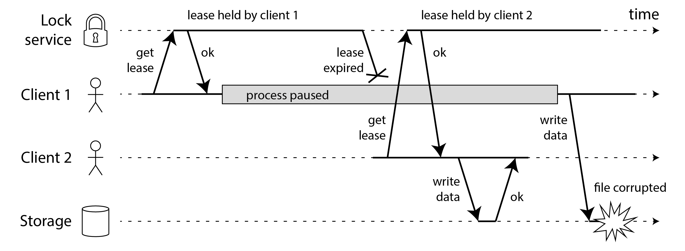
Figure 9-4 Incorrect implementation of a distributed lock: client 1 believes that it still has a valid lease, even though it has expired, and thus corrupts a file in storage.

The problem is an example of what we discussed in “Process Pauses”: if the client holding the lease is paused for too long, its lease expires. Another client can obtain a lease for the same file, and start writing to the file. When the paused client comes back, it believes (incorrectly) that it still has a valid lease and proceeds to also write to the file. We now have a split brain situation: the clients’ writes clash and corrupt the file.

Figure 9-5 shows a different problem that has similar consequences. In this example there is no process pause, only a crash by client 1. Just before client 1 crashes it sends a write request to the storage service, but this request is delayed for a long time in the network. (Remember from “Network Faults in Practice” that packets can sometimes be delayed by a minute or more.) By the time the write request arrives at the storage service, the lease has already timed out, allowing client 2 to acquire it and issue a write of its own. The result is corruption similar to Figure 9-4.

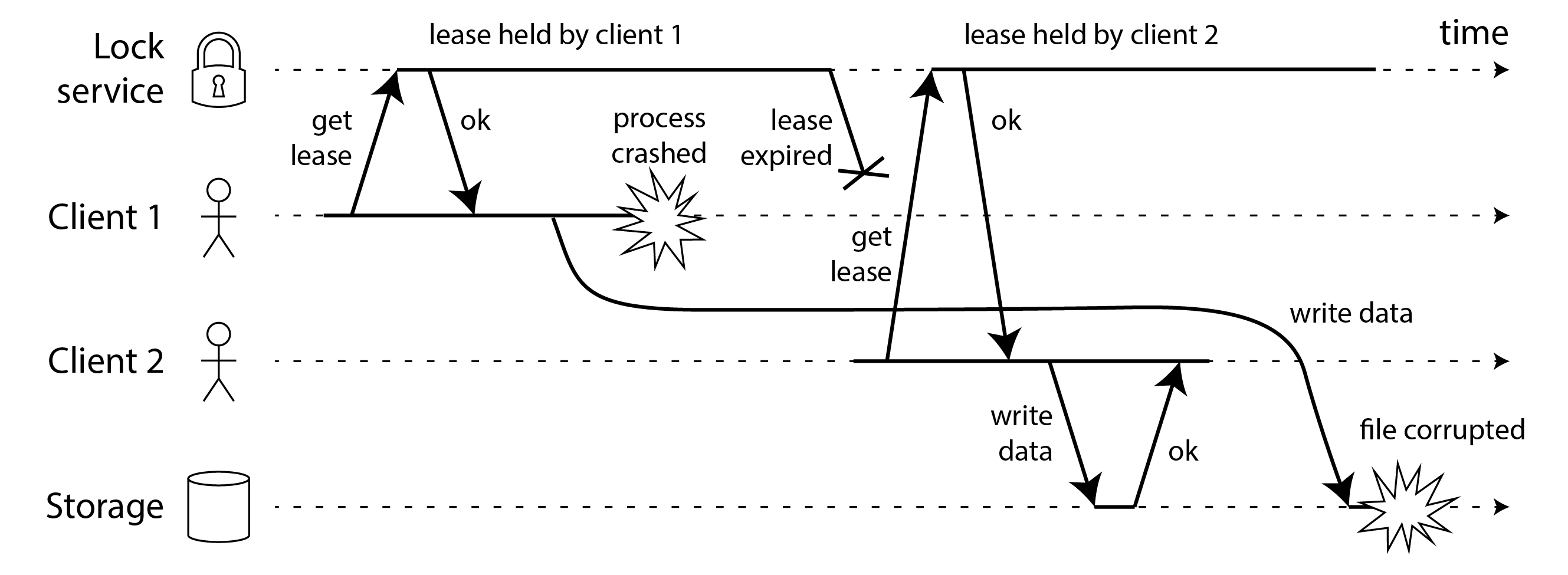
Figure 9-5 A message from a former leaseholder might be delayed for a long time, and arrive after another node has taken over the lease.

Fencing off zombies and delayed requests

The term zombie is sometimes used to describe a former leaseholder who has not yet found out that it lost the lease, and who is still acting as if it was the current leaseholder. Since we cannot rule out zombies entirely, we have to instead ensure that they can’t do any damage in the form of split brain. This is called fencing off the zombie.

Some systems attempt to fence off zombies by shutting them down, for example by disconnecting them from the network ⁹, shutting down the VM via the cloud provider’s management interface, or even physically powering down the machine ⁸⁷. This approach is known as Shoot The Other Node In The Head or STONITH. Unfortunately, it suffers from some problems: it does not protect against large network delays like in Figure 9-5; it can happen that all of the nodes shut each other down ¹⁹; and by the time the zombie has been detected and shut down, it may already be too late and data may already have been corrupted.

A more robust fencing solution, which protects against both zombies and delayed requests, is illustrated in Figure 9-6.

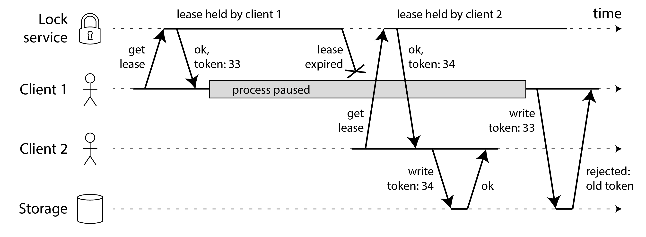
Figure 9-6 Making access to storage safe by allowing writes only in the order of increasing fencing tokens.

Let’s assume that every time the lock service grants a lock or lease, it also returns a fencing token, which is a number that increases every time a lock is granted (e.g., incremented by the lock service). We can then require that every time a client sends a write request to the storage service, it must include its current fencing token.

Note

There are several alternative names for fencing tokens. In Chubby, Google’s lock service, they are called sequencers ⁸⁸, and in Kafka they are called epoch numbers. In consensus algorithms, which we will discuss in Chapter 10, the ballot number (Paxos) or term number (Raft) serves a similar purpose.

In Figure 9-6, client 1 acquires the lease with a token of 33, but then it goes into a long pause and the lease expires. Client 2 acquires the lease with a token of 34 (the number always increases) and then sends its write request to the storage service, including the token of 34. Later, client 1 comes back to life and sends its write to the storage service, including its token value 33. However, the storage service remembers that it has already processed a write with a higher token number (34), and so it rejects the request with token 33. A client that has just acquired the lease must immediately make a write to the storage service, and once that write has completed, any zombies are fenced off.

If ZooKeeper is your lock service, you can use the transaction ID zxid or the node version cversion as fencing token ⁸⁵. With etcd, the revision number along with the lease ID serves a similar purpose ⁸⁹. The FencedLock API in Hazelcast explicitly generates a fencing token ⁹⁰.

This mechanism requires that the storage service has some way of checking whether a write is based on an outdated token. Alternatively, it’s sufficient for the service to support a write that succeeds only if the object has not been written by another client since the current client last read it, similarly to an atomic compare-and-set (CAS) operation. For example, object storage services support such a check: Amazon S3 calls it conditional writes, Azure Blob Storage calls it conditional headers, and Google Cloud Storage calls it request preconditions.

Fencing with multiple replicas

If your clients need to write only to one storage service that supports such conditional writes, the lock service is somewhat redundant ⁹¹ ⁹², since the lease assignment could have been implemented directly based on that storage service ⁹³. However, once you have a fencing token you can also use it with multiple services or replicas, and ensure that the old leaseholder is fenced off on all of those services.

For example, imagine the storage service is a leaderless replicated key-value store with last-write-wins conflict resolution (see “Leaderless Replication”). In such a system, the client sends writes directly to each replica, and each replica independently decides whether to accept a write based on a timestamp assigned by the client.

As illustrated in Figure 9-7, you can put the writer’s fencing token in the most significant bits or digits of the timestamp. You can then be sure that any timestamp generated by the new leaseholder will be greater than any timestamp from the old leaseholder, even if the old leaseholder’s writes happened later.

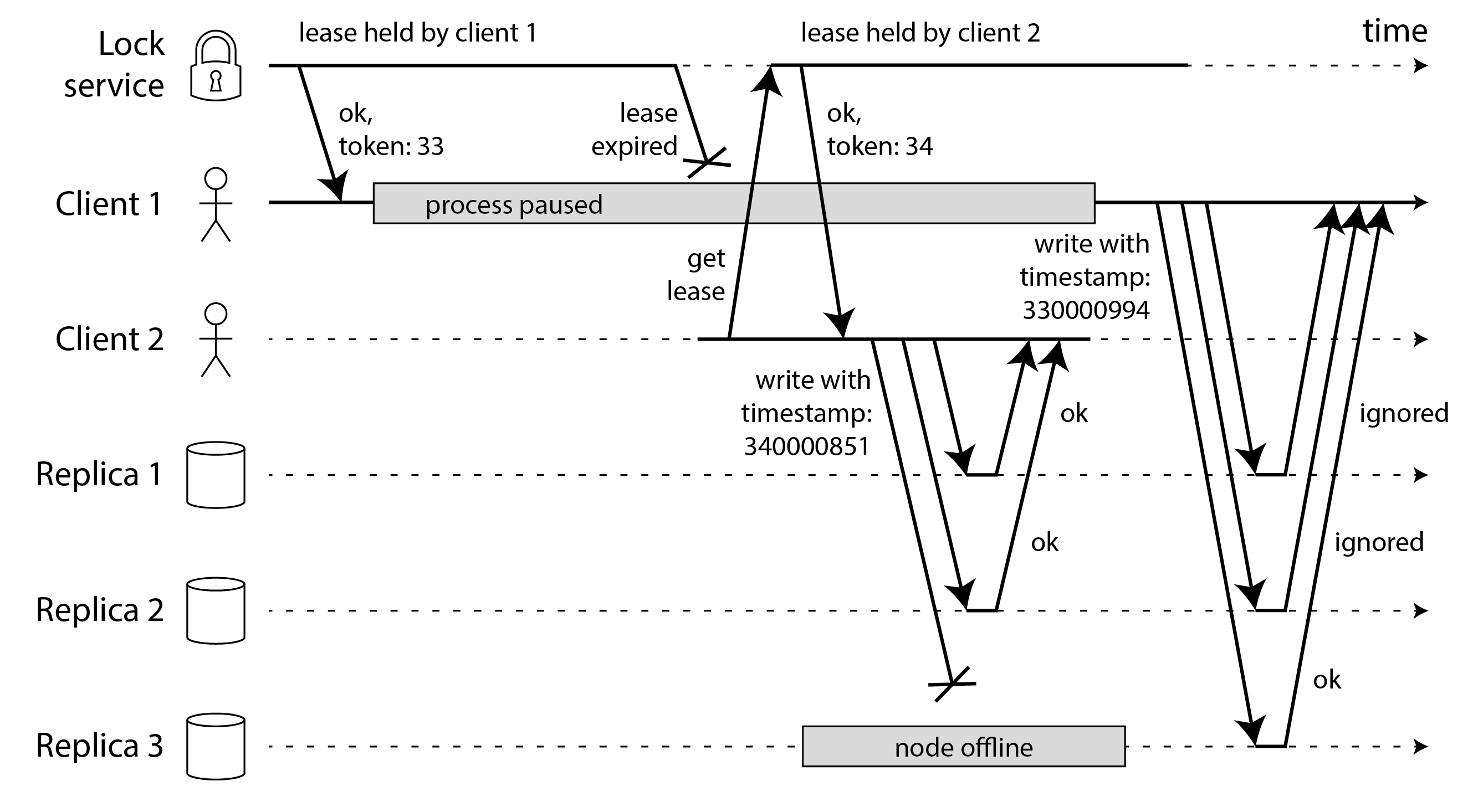
Figure 9-7 Using fencing tokens to protect writes to a leaderless replicated database.

In Figure 9-7, Client 2 has a fencing token of 34, so all of its timestamps starting with 34… are greater than any timestamps starting with 33… that are generated by Client 1. Client 2 writes to a quorum of replicas but it can’t reach Replica 3. This means that when the zombie Client 1 later tries to write, its write may succeed at Replica 3 even though it is ignored by replicas 1 and 2. This is not a problem, since a subsequent quorum read will prefer the write from Client 2 with the greater timestamp, and read repair or anti-entropy will eventually overwrite the value written by Client 1.

As you can see from these examples, it is not safe to assume that there is only one node holding a lease at any one time. Fortunately, with a bit of care you can use fencing tokens to prevent zombies and delayed requests from doing any damage.

Byzantine Faults

Fencing tokens can detect and block a node that is inadvertently acting in error (e.g., because it hasn’t yet found out that its lease has expired). However, if the node deliberately wanted to subvert the system’s guarantees, it could easily do so by sending messages with a fake fencing token.

In this book we assume that nodes are unreliable but honest: they may be slow or never respond (due to a fault), and their state may be outdated (due to a GC pause or network delays), but we assume that if a node does respond, it is telling the “truth”: to the best of its knowledge, it is playing by the rules of the protocol.

Distributed systems problems become much harder if there is a risk that nodes may “lie” (send arbitrary faulty or corrupted responses)—for example, it might cast multiple contradictory votes in the same election. Such behavior is known as a Byzantine fault, and the problem of reaching consensus in this untrusting environment is known as the Byzantine Generals Problem ⁹⁴.

THE BYZANTINE GENERALS PROBLEM

The Byzantine Generals Problem is a generalization of the so-called Two Generals Problem ⁹⁵, which imagines a situation in which two army generals need to agree on a battle plan. As they have set up camp on two different sites, they can only communicate by messenger, and the messengers sometimes get delayed or lost (like packets in a network). We will discuss this problem of consensus in Chapter 10.

In the Byzantine version of the problem, there are n generals who need to agree, and their endeavor is hampered by the fact that there are some traitors in their midst. Most of the generals are loyal, and thus send truthful messages, but the traitors may try to deceive and confuse the others by sending fake or untrue messages. It is not known in advance who the traitors are.

Byzantium was an ancient Greek city that later became Constantinople, in the place which is now Istanbul in Turkey. There isn’t any historic evidence that the generals of Byzantium were any more prone to intrigue and conspiracy than those elsewhere. Rather, the name is derived from Byzantine in the sense of excessively complicated, bureaucratic, devious, which was used in politics long before computers ⁹⁶. Lamport wanted to choose a nationality that would not offend any readers, and he was advised that calling it The Albanian Generals Problem was not such a good idea ⁹⁷.

A system is Byzantine fault-tolerant if it continues to operate correctly even if some of the nodes are malfunctioning and not obeying the protocol, or if malicious attackers are interfering with the network. This concern is relevant in certain specific circumstances. For example:

In aerospace environments, the data in a computer’s memory or CPU register could become corrupted by radiation, leading it to respond to other nodes in arbitrarily unpredictable ways. Since a system failure would be very expensive (e.g., an aircraft crashing and killing everyone on board, or a rocket colliding with the International Space Station), flight control systems must tolerate Byzantine faults ⁹⁸ ⁹⁹.
In a system with multiple participating parties, some participants may attempt to cheat or defraud others. In such circumstances, it is not safe for a node to simply trust another node’s messages, since they may be sent with malicious intent. For example, cryptocurrencies like Bitcoin and other blockchains can be considered to be a way of getting mutually untrusting parties to agree whether a transaction happened or not, without relying on a central authority ¹⁰⁰.

However, in the kinds of systems we discuss in this book, we can usually safely assume that there are no Byzantine faults. In a datacenter, all the nodes are controlled by your organization (so they can hopefully be trusted) and radiation levels are low enough that memory corruption is not a major problem (although datacenters in orbit are being considered ¹⁰¹). Multitenant systems have mutually untrusting tenants, but they are isolated from each other using firewalls, virtualization, and access control policies, not using Byzantine fault tolerance. Protocols for making systems Byzantine fault-tolerant are quite expensive ¹⁰², and fault-tolerant embedded systems rely on support from the hardware level ⁹⁸. In most server-side data systems, the cost of deploying Byzantine fault-tolerant solutions makes them impracticable.

Web applications do need to expect arbitrary and malicious behavior of clients that are under end-user control, such as web browsers. This is why input validation, sanitization, and output escaping are so important: to prevent SQL injection and cross-site scripting, for example. However, we typically don’t use Byzantine fault-tolerant protocols here, but simply make the server the authority on deciding what client behavior is and isn’t allowed. In peer-to-peer networks, where there is no such central authority, Byzantine fault tolerance is more relevant ¹⁰³ ¹⁰⁴.

A bug in the software could be regarded as a Byzantine fault, but if you deploy the same software to all nodes, then a Byzantine fault-tolerant algorithm cannot save you. Most Byzantine fault-tolerant algorithms require a supermajority of more than two-thirds of the nodes to be functioning correctly (for example, if you have four nodes, at most one may malfunction). To use this approach against bugs, you would have to have four independent implementations of the same software and hope that a bug only appears in one of the four implementations.

Similarly, it would be appealing if a protocol could protect us from vulnerabilities, security compromises, and malicious attacks. Unfortunately, this is not realistic either: in most systems, if an attacker can compromise one node, they can probably compromise all of them, because they are probably running the same software. Thus, traditional mechanisms (authentication, access control, encryption, firewalls, and so on) continue to be the main protection against attackers.

Weak forms of lying

Although we assume that nodes are generally honest, it can be worth adding mechanisms to software that guard against weak forms of “lying”—for example, invalid messages due to hardware issues, software bugs, and misconfiguration. Such protection mechanisms are not full-blown Byzantine fault tolerance, as they would not withstand a determined adversary, but they are nevertheless simple and pragmatic steps toward better reliability. For example:

Network packets do sometimes get corrupted due to hardware issues or bugs in operating systems, drivers, routers, etc. Usually, corrupted packets are caught by the checksums built into TCP and UDP, but sometimes they evade detection ¹⁰⁵ ¹⁰⁶ ¹⁰⁷. Simple measures are usually sufficient protection against such corruption, such as checksums in the application-level protocol. TLS-encrypted connections also offer protection against corruption.
A publicly accessible application must carefully sanitize any inputs from users, for example checking that a value is within a reasonable range and limiting the size of strings to prevent denial of service through large memory allocations. An internal service behind a firewall may be able to get away with less strict checks on inputs, but basic checks in protocol parsers are still a good idea ¹⁰⁵.
NTP clients can be configured with multiple server addresses. When synchronizing, the client contacts all of them, estimates their errors, and checks that a majority of servers agree on some time range. As long as most of the servers are okay, a misconfigured NTP server that is reporting an incorrect time is detected as an outlier and is excluded from synchronization ³⁹. The use of multiple servers makes NTP more robust than if it only uses a single server.

System Model and Reality

Many algorithms have been designed to solve distributed systems problems—for example, we will examine solutions for the consensus problem in Chapter 10. In order to be useful, these algorithms need to tolerate the various faults of distributed systems that we discussed in this chapter.

Algorithms need to be written in a way that does not depend too heavily on the details of the hardware and software configuration on which they are run. This in turn requires that we somehow formalize the kinds of faults that we expect to happen in a system. We do this by defining a system model, which is an abstraction that describes what things an algorithm may assume.

With regard to timing assumptions, three system models are in common use:

Synchronous model: The synchronous model assumes bounded network delay, bounded process pauses, and bounded clock error. This does not imply exactly synchronized clocks or zero network delay; it just means you know that network delay, pauses, and clock drift will never exceed some fixed upper bound ¹⁰⁸. The synchronous model is not a realistic model of most practical systems, because (as discussed in this chapter) unbounded delays and pauses do occur.
Partially synchronous model: Partial synchrony means that a system behaves like a synchronous system most of the time, but it sometimes exceeds the bounds for network delay, process pauses, and clock drift ¹⁰⁸. This is a realistic model of many systems: most of the time, networks and processes are quite well behaved—otherwise we would never be able to get anything done—but we have to reckon with the fact that any timing assumptions may be shattered occasionally. When this happens, network delay, pauses, and clock error may become arbitrarily large.
Asynchronous model: In this model, an algorithm is not allowed to make any timing assumptions—in fact, it does not even have a clock (so it cannot use timeouts). Some algorithms can be designed for the asynchronous model, but it is very restrictive.

Moreover, besides timing issues, we have to consider node failures. Some common system models for nodes are:

Crash-stop faults: In the crash-stop (or fail-stop) model, an algorithm may assume that a node can fail in only one way, namely by crashing ¹⁰⁹. This means that the node may suddenly stop responding at any moment, and thereafter that node is gone forever—it never comes back.
Crash-recovery faults: We assume that nodes may crash at any moment, and perhaps start responding again after some unknown time. In the crash-recovery model, nodes are assumed to have stable storage (i.e., nonvolatile disk storage) that is preserved across crashes, while the in-memory state is assumed to be lost.
Degraded performance and partial functionality: In addition to crashing and restarting, nodes may go slow: they may still be able to respond to health check requests, while being too slow to get any real work done. For example, a Gigabit network interface could suddenly drop to 1 Kb/s throughput due to a driver bug ¹¹⁰; a process that is under memory pressure may spend most of its time performing garbage collection ¹¹¹; worn-out SSDs can have erratic performance; and hardware can be affected by high temperature, loose connectors, mechanical vibration, power supply problems, firmware bugs, and more ¹¹². Such a situation is called a limping node, gray failure, or fail-slow ¹¹³, and it can be even more difficult to deal with than a cleanly failed node. A related problem is when a process stops doing some of the things it is supposed to do while other aspects continue working, for example because a background thread is crashed or deadlocked ¹¹⁴.
Byzantine (arbitrary) faults: Nodes may do absolutely anything, including trying to trick and deceive other nodes, as described in the last section.

For modeling real systems, the partially synchronous model with crash-recovery faults is generally the most useful model. It allows for unbounded network delay, process pauses, and slow nodes. But how do distributed algorithms cope with that model?

Defining the correctness of an algorithm

To define what it means for an algorithm to be correct, we can describe its properties. For example, the output of a sorting algorithm has the property that for any two distinct elements of the output list, the element further to the left is smaller than the element further to the right. That is simply a formal way of defining what it means for a list to be sorted.

Similarly, we can write down the properties we want of a distributed algorithm to define what it means to be correct. For example, if we are generating fencing tokens for a lock (see “Fencing off zombies and delayed requests”), we may require the algorithm to have the following properties:

Uniqueness: No two requests for a fencing token return the same value.
Monotonic sequence: If request x returned token t_x, and request y returned token t_y, and x completed before y began, then t_x < t_y.
Availability: A node that requests a fencing token and does not crash eventually receives a response.

An algorithm is correct in some system model if it always satisfies its properties in all situations that we assume may occur in that system model. However, if all nodes crash, or all network delays suddenly become infinitely long, then no algorithm will be able to get anything done. How can we still make useful guarantees even in a system model that allows complete failures?

Safety and liveness

To clarify the situation, it is worth distinguishing between two different kinds of properties: safety and liveness properties. In the example just given, uniqueness and monotonic sequence are safety properties, but availability is a liveness property.

What distinguishes the two kinds of properties? A giveaway is that liveness properties often include the word “eventually” in their definition. (And yes, you guessed it—eventual consistency is a liveness property ¹¹⁵.)

Safety is often informally defined as nothing bad happens, and liveness as something good eventually happens. However, it’s best to not read too much into those informal definitions, because “good” and “bad” are value judgements that don’t apply well to algorithms. The actual definitions of safety and liveness are more precise ¹¹⁶:

If a safety property is violated, we can point at a particular point in time at which it was broken (for example, if the uniqueness property was violated, we can identify the particular operation in which a duplicate fencing token was returned). After a safety property has been violated, the violation cannot be undone—the damage is already done.
A liveness property works the other way round: it may not hold at some point in time (for example, a node may have sent a request but not yet received a response), but there is always hope that it may be satisfied in the future (namely by receiving a response).

An advantage of distinguishing between safety and liveness properties is that it helps us deal with difficult system models. For distributed algorithms, it is common to require that safety properties always hold, in all possible situations of a system model ¹⁰⁸. That is, even if all nodes crash, or the entire network fails, the algorithm must nevertheless ensure that it does not return a wrong result (i.e., that the safety properties remain satisfied).

However, with liveness properties we are allowed to make caveats: for example, we could say that a request needs to receive a response only if a majority of nodes have not crashed, and only if the network eventually recovers from an outage. The definition of the partially synchronous model requires that eventually the system returns to a synchronous state—that is, any period of network interruption lasts only for a finite duration and is then repaired.

Mapping system models to the real world

Safety and liveness properties and system models are very useful for reasoning about the correctness of a distributed algorithm. However, when implementing an algorithm in practice, the messy facts of reality come back to bite you again, and it becomes clear that the system model is a simplified abstraction of reality.

For example, algorithms in the crash-recovery model generally assume that data in stable storage survives crashes. However, what happens if the data on disk is corrupted, or the data is wiped out due to hardware error or misconfiguration ¹¹⁷? What happens if a server has a firmware bug and fails to recognize its hard drives on reboot, even though the drives are correctly attached to the server ¹¹⁸?

Quorum algorithms (see “Quorums for reading and writing”) rely on a node remembering the data that it claims to have stored. If a node may suffer from amnesia and forget previously stored data, that breaks the quorum condition, and thus breaks the correctness of the algorithm. Perhaps a new system model is needed, in which we assume that stable storage mostly survives crashes, but may sometimes be lost. But that model then becomes harder to reason about.

The theoretical description of an algorithm can declare that certain things are simply assumed not to happen—and in non-Byzantine systems, we do have to make some assumptions about faults that can and cannot happen. However, a real implementation may still have to include code to handle the case where something happens that was assumed to be impossible, even if that handling boils down to printf("Sucks to be you") and exit(666)—i.e., letting a human operator clean up the mess ¹¹⁹. (This is one difference between computer science and software engineering.)

That is not to say that theoretical, abstract system models are worthless—quite the opposite. They are incredibly helpful for distilling down the complexity of real systems to a manageable set of faults that we can reason about, so that we can understand the problem and try to solve it systematically.

Formal Methods and Randomized Testing

How do we know that an algorithm satisfies the required properties? Due to concurrency, partial failures, and network delays there are a huge number of potential states. We need to guarantee that the properties hold in every possible state, and ensure that we haven’t forgotten about any edge cases.

One approach is to formally verify an algorithm by describing it mathematically, and using proof techniques to show that it satisfies the required properties in all situations that the system model allows. Proving an algorithm correct does not mean its implementation on a real system will necessarily always behave correctly. But it’s a very good first step, because the theoretical analysis can uncover problems in an algorithm that might remain hidden for a long time in a real system, and that only come to bite you when your assumptions (e.g., about timing) are defeated due to unusual circumstances.

It is prudent to combine theoretical analysis with empirical testing to verify that implementations behave as expected. Techniques such as property-based testing, fuzzing, and deterministic simulation testing (DST) use randomization to test a system in a wide range of situations. Companies such as Amazon Web Services have successfully used a combination of these techniques on many of their products ¹²⁰ ¹²¹.

Model checking and specification languages

Model checkers are tools that help verify that an algorithm or system behaves as expected. An algorithm specification is written in a purpose-built language such as TLA+, Gallina, or FizzBee. These languages make it easier to focus on an algorithm’s behavior without worrying about code implementation details. Model checkers then use these models to verify that invariants hold across all of an algorithm’s states by systematically trying all the things that could happen.

Model checking can’t actually prove that an algorithm’s invariants hold for every possible state since most real-world algorithms have an infinite state space. A true verification of all states would require a formal proof, which can be done, but which is typically more difficult than running a model checker. Instead, model checkers encourage you to reduce the algorithm’s model to an approximation that can be fully verified, or to limit the execution to some upper bound (for example, by setting a maximum number of messages that can be sent). Any bugs that only occur with longer executions would then not be found.

Still, model checkers strike a nice balance between ease of use and the ability to find non-obvious bugs. CockroachDB, TiDB, Kafka, and many other distributed systems use model specifications to find and fix bugs ¹²² ¹²³ ¹²⁴. For example, using TLA+, researchers were able to demonstrate the potential for data loss in viewstamped replication (VR) caused by ambiguity in the prose description of the algorithm ¹²⁵.

By design, model checkers don’t run your actual code, but rather a simplified model that specifies only the core ideas of your protocol. This makes it more tractable to systematically explore the state space, but it risks that your specification and your implementation go out of sync with each other ¹²⁶. It is possible to check whether the model and the real implementation have equivalent behavior, but this requires instrumentation in the real implementation ¹²⁷.

Fault injection

Many bugs are triggered when machine and network failures occur. Fault injection is an effective (and sometimes scary) technique that verifies whether a system’s implementation works as expected things go wrong. The idea is simple: inject faults into a running system’s environment and see how it behaves. Faults can be network failures, machine crashes, disk corruption, paused processes—anything you can imagine going wrong with a computer.

Fault injection tests are typically run in an environment that closely resembles the production environment where the system will run. Some even inject faults directly into their production environment. Netflix popularized this approach with their Chaos Monkey tool ¹²⁸. Production fault injection is often referred to as chaos engineering, which we discussed in “Reliability and Fault Tolerance”.

To run fault injection tests, the system under test is first deployed along with fault injection coordinators and scripts. Coordinators are responsible for deciding what faults to execute and when to execute them. Local or remote scripts are responsible for injecting failures into individual nodes or processes. Injection scripts use many different tools to trigger faults. A Linux process can be paused or killed using Linux’s kill command, a disk can be unmounted with umount, and network connections can be disrupted through firewall settings. You can inspect system behavior during and after faults are injected to make sure things work as expected.

The myriad of tools required to trigger failures make fault injection tests cumbersome to write. It’s common to adopt a fault injection framework like Jepsen to run fault injection tests to simplify the process. Such frameworks come with integrations for various operating systems and many pre-built fault injectors ¹²⁹. Jepsen has been remarkably effective at finding critical bugs in many widely-used systems ¹³⁰ ¹³¹.

Deterministic simulation testing

Deterministic simulation testing (DST) has also become a popular complement to model-checking and fault injection. It uses a similar state space exploration process as a model checker, but it tests your actual code, not a model.

In DST, a simulation automatically runs through a large number of randomised executions of the system. Network communication, I/O, and clock timing during the simulation are all replaced with mocks that allow the simulator to control the exact order in which things happen, including various timings and failure scenarios. This allows the simulator to explore many more situations than hand-written tests or fault injection could. If a test fails, it can be re-run since the simulator knows the exact order of operations that triggered the failure—in contrast to fault injection, which does not have such fine-grained control over the system.

DST requires the simulator to be able to control all sources of nondeterminism, such as network delays. One of three strategies is generally adopted to make code deterministic:

Application-level: Some systems are built from the ground-up to make it easy to execute code deterministically. For example, FoundationDB, one of the pioneers in the DST space, is built using an asynchronous communication library called Flow. Flow provides a point for developers to inject a deterministic network simulation into the system ¹³². Similarly, TigerBeetle is an online transaction processing (OLTP) database with first-class DST support. The system’s state is modeled as a state machine, with all mutations occuring within a single event loop. When combined with mock deterministic primitives such as clocks, such an architecture is able to run deterministically ¹³³.
Runtime-level: Languages with asynchronous runtimes and commonly used libraries provide an insertion point to introduce determinism. A single-threaded runtime is used to force all asynchronous code to run sequentially. FrostDB, for example, patches Go’s runtime to execute goroutines sequentially ¹³⁴. Rust’s madsim library works in a similar manner. Madsim provides deterministic implementations of Tokio’s asynchronous runtime API, AWS’s S3 library, Kafka’s Rust library, and many others. Applications can swap in deterministic libraries and runtimes to get deterministic test executions without changing their code.
Machine-level: Rather than patching code at runtime, an entire machine can be made deterministic. This is a delicate process that requires a machine to respond to all normally nondeterministic calls with deterministic responses. Tools such as Antithesis do this by building a custom hypervisor that replaces normally nondeterministic operations with deterministic ones. Everything from clocks to network and storage needs to be accounted for. Once done, though, developers can run their entire distributed system in a collection of containers within the hypervisor and get a completely deterministic distributed system.

DST provides several advantages beyond replayability. Tools such as Antithesis attempt to explore many different code paths in application code by branching a test execution into multiple sub-executions when it discovers less common behavior. And because deterministic tests often use mocked clocks and network calls, such tests can run faster than wall-clock time. For example, TigerBeetle’s time abstraction allows simulations to simulate network latency and timeouts without actually taking the full length of time to trigger the timeout. Such techniques allow the simulator to explore more code paths faster.

The Power of Determinism

Nondeterminism is at the core of all of the distributed systems challenges we discussed in this chapter: concurrency, network delay, process pauses, clock jumps, and crashes all happen in unpredictable ways that vary from one run of a system to the next. Conversely, if you can make a system deterministic, that can hugely simplify things.

In fact, making things deterministic is a simple but powerful idea that arises again and again in distributed system design. Besides deterministic simulation testing, we have seen several ways of using determinism over the past chapters:

A key advantage of event sourcing (see “Event Sourcing and CQRS”) is that you can deterministically replay a log of events to reconstruct derived materialized views.
Workflow engines (see “Durable Execution and Workflows”) rely on workflow definitions being deterministic to provide durable execution semantics.
State machine replication, which we will discuss in “Using shared logs”, replicates data by independently executing the same sequence of deterministic transactions on each replica. We have already seen two variants of that idea: statement-based replication (see “Implementation of Replication Logs”) and serial transaction execution using stored procedures (see “Pros and cons of stored procedures”).

However, making code fully deterministic requires care. Even once you have removed all concurrency and replaced I/O, network communication, clocks, and random number generators with deterministic simulations, elements of nondeterminism may remain. For example, in some programming languages, the order in which you iterate over the elements of a hash table may be nondeterministic. Whether you run into a resource limit (memory allocation failure, stack overflow) is also nondeterministic.

Summary

In this chapter we have discussed a wide range of problems that can occur in distributed systems, including:

Whenever you try to send a packet over the network, it may be lost or arbitrarily delayed. Likewise, the reply may be lost or delayed, so if you don’t get a reply, you have no idea whether the message got through.
A node’s clock may be significantly out of sync with other nodes (despite your best efforts to set up NTP), it may suddenly jump forward or back in time, and relying on it is dangerous because you most likely don’t have a good measure of your clock’s confidence interval.
A process may pause for a substantial amount of time at any point in its execution, be declared dead by other nodes, and then come back to life again without realizing that it was paused.

The fact that such partial failures can occur is the defining characteristic of distributed systems. Whenever software tries to do anything involving other nodes, there is the possibility that it may occasionally fail, or randomly go slow, or not respond at all (and eventually time out). In distributed systems, we try to build tolerance of partial failures into software, so that the system as a whole may continue functioning even when some of its constituent parts are broken.

To tolerate faults, the first step is to detect them, but even that is hard. Most systems don’t have an accurate mechanism of detecting whether a node has failed, so most distributed algorithms rely on timeouts to determine whether a remote node is still available. However, timeouts can’t distinguish between network and node failures, and variable network delay sometimes causes a node to be falsely suspected of crashing. Handling limping nodes, which are responding but are too slow to do anything useful, is even harder.

Once a fault is detected, making a system tolerate it is not easy either: there is no global variable, no shared memory, no common knowledge or any other kind of shared state between the machines ⁸³. Nodes can’t even agree on what time it is, let alone on anything more profound. The only way information can flow from one node to another is by sending it over the unreliable network. Major decisions cannot be safely made by a single node, so we require protocols that enlist help from other nodes and try to get a quorum to agree.

If you’re used to writing software in the idealized mathematical perfection of a single computer, where the same operation always deterministically returns the same result, then moving to the messy physical reality of distributed systems can be a bit of a shock. Conversely, distributed systems engineers will often regard a problem as trivial if it can be solved on a single computer ⁴, and indeed a single computer can do a lot nowadays. If you can avoid opening Pandora’s box and simply keep things on a single machine, for example by using an embedded storage engine (see “Embedded storage engines”), it is generally worth doing so.

However, as discussed in “Distributed versus Single-Node Systems”, scalability is not the only reason for wanting to use a distributed system. Fault tolerance and low latency (by placing data geographically close to users) are equally important goals, and those things cannot be achieved with a single node. The power of distributed systems is that in principle, they can run forever without being interrupted at the service level, because all faults and maintenance can be handled at the node level. (In practice, if a bad configuration change is rolled out to all nodes, that will still bring a distributed system to its knees.)

In this chapter we also went on some tangents to explore whether the unreliability of networks, clocks, and processes is an inevitable law of nature. We saw that it isn’t: it is possible to give hard real-time response guarantees and bounded delays in networks, but doing so is very expensive and results in lower utilization of hardware resources. Most non-safety-critical systems choose cheap and unreliable over expensive and reliable.

This chapter has been all about problems, and has given us a bleak outlook. In the next chapter we will move on to solutions, and discuss some algorithms that have been designed to cope with the problems in distributed systems.

References

Mark Cavage. There’s Just No Getting Around It: You’re Building a Distributed System. ACM Queue, volume 11, issue 4, pages 80-89, April 2013. doi:10.1145/2466486.2482856 ↩︎
Jay Kreps. Getting Real About Distributed System Reliability. blog.empathybox.com, March 2012. Archived at perma.cc/9B5Q-AEBW ↩︎
Coda Hale. You Can’t Sacrifice Partition Tolerance. codahale.com, October 2010. https://perma.cc/6GJU-X4G5 ↩︎
Jeff Hodges. Notes on Distributed Systems for Young Bloods. somethingsimilar.com, January 2013. Archived at perma.cc/B636-62CE ↩︎ ↩︎
Van Jacobson. Congestion Avoidance and Control. At ACM Symposium on Communications Architectures and Protocols (SIGCOMM), August 1988. doi:10.1145/52324.52356 ↩︎ ↩︎
Bert Hubert. The Ultimate SO_LINGER Page, or: Why Is My TCP Not Reliable. blog.netherlabs.nl, January 2009. Archived at perma.cc/6HDX-L2RR ↩︎ ↩︎
Jerome H. Saltzer, David P. Reed, and David D. Clark. End-To-End Arguments in System Design. ACM Transactions on Computer Systems, volume 2, issue 4, pages 277–288, November 1984. doi:10.1145/357401.357402 ↩︎
Peter Bailis and Kyle Kingsbury. The Network Is Reliable. ACM Queue, volume 12, issue 7, pages 48-55, July 2014. doi:10.1145/2639988.2639988 ↩︎ ↩︎
Joshua B. Leners, Trinabh Gupta, Marcos K. Aguilera, and Michael Walfish. Taming Uncertainty in Distributed Systems with Help from the Network. At 10th European Conference on Computer Systems (EuroSys), April 2015. doi:10.1145/2741948.2741976 ↩︎ ↩︎
Phillipa Gill, Navendu Jain, and Nachiappan Nagappan. Understanding Network Failures in Data Centers: Measurement, Analysis, and Implications. At ACM SIGCOMM Conference, August 2011. doi:10.1145/2018436.2018477 ↩︎
Urs Hölzle. But recently a farmer had started grazing a herd of cows nearby. And whenever they stepped on the fiber link, they bent it enough to cause a blip. x.com, May 2020. Archived at perma.cc/WX8X-ZZA5 ↩︎
CBC News. Hundreds lose internet service in northern B.C. after beaver chews through cable. cbc.ca, April 2021. Archived at perma.cc/UW8C-H2MY ↩︎
Will Oremus. The Global Internet Is Being Attacked by Sharks, Google Confirms. slate.com, August 2014. Archived at perma.cc/P6F3-C6YG ↩︎
Jess Auerbach Jahajeeah. Down to the wire: The ship fixing our internet. continent.substack.com, November 2023. Archived at perma.cc/DP7B-EQ7S ↩︎
Santosh Janardhan. More details about the October 4 outage. engineering.fb.com, October 2021. Archived at perma.cc/WW89-VSXH ↩︎
Tom Parfitt. Georgian woman cuts off web access to whole of Armenia. theguardian.com, April 2011. Archived at perma.cc/KMC3-N3NZ ↩︎
Antonio Voce, Tural Ahmedzade and Ashley Kirk. ‘Shadow fleets’ and subaquatic sabotage: are Europe’s undersea internet cables under attack? theguardian.com, March 2025. Archived at perma.cc/HA7S-ZDBV ↩︎
Shengyun Liu, Paolo Viotti, Christian Cachin, Vivien Quéma, and Marko Vukolić. XFT: Practical Fault Tolerance beyond Crashes. At 12th USENIX Symposium on Operating Systems Design and Implementation (OSDI), November 2016. ↩︎
Mark Imbriaco. Downtime last Saturday. github.blog, December 2012. Archived at perma.cc/M7X5-E8SQ ↩︎ ↩︎
Tom Lianza and Chris Snook. A Byzantine failure in the real world. blog.cloudflare.com, November 2020. Archived at perma.cc/83EZ-ALCY ↩︎ ↩︎
Mohammed Alfatafta, Basil Alkhatib, Ahmed Alquraan, and Samer Al-Kiswany. Toward a Generic Fault Tolerance Technique for Partial Network Partitioning. At 14th USENIX Symposium on Operating Systems Design and Implementation (OSDI), November 2020. ↩︎
Marc A. Donges. Re: bnx2 cards Intermittantly Going Offline. Message to Linux netdev mailing list, spinics.net, September 2012. Archived at perma.cc/TXP6-H8R3 ↩︎ ↩︎
Troy Toman. Inside a CODE RED: Network Edition. signalvnoise.com, September 2020. Archived at perma.cc/BET6-FY25 ↩︎
Kyle Kingsbury. Call Me Maybe: Elasticsearch. aphyr.com, June 2014. perma.cc/JK47-S89J ↩︎
Salvatore Sanfilippo. A Few Arguments About Redis Sentinel Properties and Fail Scenarios. antirez.com, October 2014. perma.cc/8XEU-CLM8 ↩︎
Nicolas Liochon. CAP: If All You Have Is a Timeout, Everything Looks Like a Partition. blog.thislongrun.com, May 2015. Archived at perma.cc/FS57-V2PZ ↩︎
Matthew P. Grosvenor, Malte Schwarzkopf, Ionel Gog, Robert N. M. Watson, Andrew W. Moore, Steven Hand, and Jon Crowcroft. Queues Don’t Matter When You Can JUMP Them! At 12th USENIX Symposium on Networked Systems Design and Implementation (NSDI), May 2015. ↩︎ ↩︎
Theo Julienne. Debugging network stalls on Kubernetes. github.blog, November 2019. Archived at perma.cc/K9M8-XVGL ↩︎
Guohui Wang and T. S. Eugene Ng. The Impact of Virtualization on Network Performance of Amazon EC2 Data Center. At 29th IEEE International Conference on Computer Communications (INFOCOM), March 2010. doi:10.1109/INFCOM.2010.5461931 ↩︎ ↩︎
Brandon Philips. etcd: Distributed Locking and Service Discovery. At Strange Loop, September 2014. ↩︎
Steve Newman. A Systematic Look at EC2 I/O. blog.scalyr.com, October 2012. Archived at perma.cc/FL4R-H2VE ↩︎ ↩︎
Naohiro Hayashibara, Xavier Défago, Rami Yared, and Takuya Katayama. The ϕ Accrual Failure Detector. Japan Advanced Institute of Science and Technology, School of Information Science, Technical Report IS-RR-2004-010, May 2004. Archived at perma.cc/NSM2-TRYA ↩︎
Jeffrey Wang. Phi Accrual Failure Detector. ternarysearch.blogspot.co.uk, August 2013. perma.cc/L452-AMLV ↩︎
Srinivasan Keshav. An Engineering Approach to Computer Networking: ATM Networks, the Internet, and the Telephone Network. Addison-Wesley Professional, May 1997. ISBN: 978-0-201-63442-6 ↩︎ ↩︎
Othmar Kyas. ATM Networks. International Thomson Publishing, 1995. ISBN: 978-1-850-32128-6 ↩︎
Mellanox Technologies. InfiniBand FAQ, Rev 1.3. network.nvidia.com, December 2014. Archived at perma.cc/LQJ4-QZVK ↩︎
Jose Renato Santos, Yoshio Turner, and G. (John) Janakiraman. End-to-End Congestion Control for InfiniBand. At 22nd Annual Joint Conference of the IEEE Computer and Communications Societies (INFOCOM), April 2003. Also published by HP Laboratories Palo Alto, Tech Report HPL-2002-359. doi:10.1109/INFCOM.2003.1208949 ↩︎
Jialin Li, Naveen Kr. Sharma, Dan R. K. Ports, and Steven D. Gribble. Tales of the Tail: Hardware, OS, and Application-level Sources of Tail Latency. At ACM Symposium on Cloud Computing (SOCC), November 2014. doi:10.1145/2670979.2670988 ↩︎
Ulrich Windl, David Dalton, Marc Martinec, and Dale R. Worley. The NTP FAQ and HOWTO. ntp.org, November 2006. ↩︎ ↩︎ ↩︎
John Graham-Cumming. How and why the leap second affected Cloudflare DNS. blog.cloudflare.com, January 2017. Archived at archive.org ↩︎ ↩︎
David Holmes. Inside the Hotspot VM: Clocks, Timers and Scheduling Events – Part I – Windows. blogs.oracle.com, October 2006. Archived at archive.org ↩︎
Joran Dirk Greef. Three Clocks are Better than One. tigerbeetle.com, August 2021. Archived at perma.cc/5RXG-EU6B ↩︎
Oliver Yang. Pitfalls of TSC usage. oliveryang.net, September 2015. Archived at perma.cc/Z2QY-5FRA ↩︎
Steve Loughran. Time on Multi-Core, Multi-Socket Servers. steveloughran.blogspot.co.uk, September 2015. Archived at perma.cc/7M4S-D4U6 ↩︎
James C. Corbett, Jeffrey Dean, Michael Epstein, Andrew Fikes, Christopher Frost, JJ Furman, Sanjay Ghemawat, Andrey Gubarev, Christopher Heiser, Peter Hochschild, Wilson Hsieh, Sebastian Kanthak, Eugene Kogan, Hongyi Li, Alexander Lloyd, Sergey Melnik, David Mwaura, David Nagle, Sean Quinlan, Rajesh Rao, Lindsay Rolig, Dale Woodford, Yasushi Saito, Christopher Taylor, Michal Szymaniak, and Ruth Wang. Spanner: Google’s Globally-Distributed Database. At 10th USENIX Symposium on Operating System Design and Implementation (OSDI), October 2012. ↩︎ ↩︎ ↩︎
M. Caporaloni and R. Ambrosini. How Closely Can a Personal Computer Clock Track the UTC Timescale Via the Internet? European Journal of Physics, volume 23, issue 4, pages L17–L21, June 2012. doi:10.1088/0143-0807/23/4/103 ↩︎
Nelson Minar. A Survey of the NTP Network. alumni.media.mit.edu, December 1999. Archived at perma.cc/EV76-7ZV3 ↩︎
Viliam Holub. Synchronizing Clocks in a Cassandra Cluster Pt. 1 – The Problem. blog.rapid7.com, March 2014. Archived at perma.cc/N3RV-5LNL ↩︎
Poul-Henning Kamp. The One-Second War (What Time Will You Die?) ACM Queue, volume 9, issue 4, pages 44–48, April 2011. doi:10.1145/1966989.1967009 ↩︎
Nelson Minar. Leap Second Crashes Half the Internet. somebits.com, July 2012. Archived at perma.cc/2WB8-D6EU ↩︎
Christopher Pascoe. Time, Technology and Leaping Seconds. googleblog.blogspot.co.uk, September 2011. Archived at perma.cc/U2JL-7E74 ↩︎
Mingxue Zhao and Jeff Barr. Look Before You Leap – The Coming Leap Second and AWS. aws.amazon.com, May 2015. Archived at perma.cc/KPE9-XMFM ↩︎
Darryl Veitch and Kanthaiah Vijayalayan. Network Timing and the 2015 Leap Second. At 17th International Conference on Passive and Active Measurement (PAM), April 2016. doi:10.1007/978-3-319-30505-9_29 ↩︎
VMware, Inc. Timekeeping in VMware Virtual Machines. vmware.com, October 2008. Archived at perma.cc/HM5R-T5NF ↩︎
Victor Yodaiken. Clock Synchronization in Finance and Beyond. yodaiken.com, November 2017. Archived at perma.cc/9XZD-8ZZN ↩︎
Mustafa Emre Acer, Emily Stark, Adrienne Porter Felt, Sascha Fahl, Radhika Bhargava, Bhanu Dev, Matt Braithwaite, Ryan Sleevi, and Parisa Tabriz. Where the Wild Warnings Are: Root Causes of Chrome HTTPS Certificate Errors. At ACM SIGSAC Conference on Computer and Communications Security (CCS), pages 1407–1420, October 2017. doi:10.1145/3133956.3134007 ↩︎
European Securities and Markets Authority. MiFID II / MiFIR: Regulatory Technical and Implementing Standards – Annex I. esma.europa.eu, Report ESMA/2015/1464, September 2015. Archived at perma.cc/ZLX9-FGQ3 ↩︎
Luke Bigum. Solving MiFID II Clock Synchronisation With Minimum Spend (Part 1). catach.blogspot.com, November 2015. Archived at perma.cc/4J5W-FNM4 ↩︎
Oleg Obleukhov and Ahmad Byagowi. How Precision Time Protocol is being deployed at Meta. engineering.fb.com, November 2022. Archived at perma.cc/29G6-UJNW ↩︎
John Wiseman. gpsjam.org, July 2022. ↩︎
Josh Levinson, Julien Ridoux, and Chris Munns. It’s About Time: Microsecond-Accurate Clocks on Amazon EC2 Instances. aws.amazon.com, November 2023. Archived at perma.cc/56M6-5VMZ ↩︎
Kyle Kingsbury. Call Me Maybe: Cassandra. aphyr.com, September 2013. Archived at perma.cc/4MBR-J96V ↩︎ ↩︎ ↩︎
John Daily. Clocks Are Bad, or, Welcome to the Wonderful World of Distributed Systems. riak.com, November 2013. Archived at perma.cc/4XB5-UCXY ↩︎ ↩︎
Marc Brooker. It’s About Time! brooker.co.za, November 2023. Archived at perma.cc/N6YK-DRPA ↩︎
Kyle Kingsbury. The Trouble with Timestamps. aphyr.com, October 2013. Archived at perma.cc/W3AM-5VAV ↩︎
Leslie Lamport. Time, Clocks, and the Ordering of Events in a Distributed System. Communications of the ACM, volume 21, issue 7, pages 558–565, July 1978. doi:10.1145/359545.359563 ↩︎
Justin Sheehy. There Is No Now: Problems With Simultaneity in Distributed Systems. ACM Queue, volume 13, issue 3, pages 36–41, March 2015. doi:10.1145/2733108 ↩︎
Murat Demirbas. Spanner: Google’s Globally-Distributed Database. muratbuffalo.blogspot.co.uk, July 2013. Archived at perma.cc/6VWR-C9WB ↩︎
Dahlia Malkhi and Jean-Philippe Martin. Spanner’s Concurrency Control. ACM SIGACT News, volume 44, issue 3, pages 73–77, September 2013. doi:10.1145/2527748.2527767 ↩︎
Franck Pachot. Achieving Precise Clock Synchronization on AWS. yugabyte.com, December 2024. Archived at perma.cc/UYM6-RNBS ↩︎
Spencer Kimball. Living Without Atomic Clocks: Where CockroachDB and Spanner diverge. cockroachlabs.com, January 2022. Archived at perma.cc/AWZ7-RXFT ↩︎
Murat Demirbas. Use of Time in Distributed Databases (part 4): Synchronized clocks in production databases. muratbuffalo.blogspot.com, January 2025. Archived at perma.cc/9WNX-Q9U3 ↩︎
Cary G. Gray and David R. Cheriton. Leases: An Efficient Fault-Tolerant Mechanism for Distributed File Cache Consistency. At 12th ACM Symposium on Operating Systems Principles (SOSP), December 1989. doi:10.1145/74850.74870 ↩︎
Daniel Sturman, Scott Delap, Max Ross, et al. Roblox Return to Service. corp.roblox.com, January 2022. Archived at perma.cc/8ALT-WAS4 ↩︎
Todd Lipcon. Avoiding Full GCs with MemStore-Local Allocation Buffers. slideshare.net, February 2011. Archived at https://perma.cc/CH62-2EWJ ↩︎
Christopher Clark, Keir Fraser, Steven Hand, Jacob Gorm Hansen, Eric Jul, Christian Limpach, Ian Pratt, and Andrew Warfield. Live Migration of Virtual Machines. At 2nd USENIX Symposium on Symposium on Networked Systems Design & Implementation (NSDI), May 2005. ↩︎
Mike Shaver. fsyncers and Curveballs. shaver.off.net, May 2008. Archived at archive.org ↩︎
Zhenyun Zhuang and Cuong Tran. Eliminating Large JVM GC Pauses Caused by Background IO Traffic. engineering.linkedin.com, February 2016. Archived at perma.cc/ML2M-X9XT ↩︎
Martin Thompson. Java Garbage Collection Distilled. mechanical-sympathy.blogspot.co.uk, July 2013. Archived at perma.cc/DJT3-NQLQ ↩︎ ↩︎
David Terei and Amit Levy. Blade: A Data Center Garbage Collector. arXiv:1504.02578, April 2015. ↩︎
Martin Maas, Tim Harris, Krste Asanović, and John Kubiatowicz. Trash Day: Coordinating Garbage Collection in Distributed Systems. At 15th USENIX Workshop on Hot Topics in Operating Systems (HotOS), May 2015. ↩︎
Martin Fowler. The LMAX Architecture. martinfowler.com, July 2011. Archived at perma.cc/5AV4-N6RJ ↩︎
Joseph Y. Halpern and Yoram Moses. Knowledge and common knowledge in a distributed environment. Journal of the ACM (JACM), volume 37, issue 3, pages 549–587, July 1990. doi:10.1145/79147.79161 ↩︎ ↩︎
Chuzhe Tang, Zhaoguo Wang, Xiaodong Zhang, Qianmian Yu, Binyu Zang, Haibing Guan, and Haibo Chen. Ad Hoc Transactions in Web Applications: The Good, the Bad, and the Ugly. At ACM International Conference on Management of Data (SIGMOD), June 2022. doi:10.1145/3514221.3526120 ↩︎
Flavio P. Junqueira and Benjamin Reed. ZooKeeper: Distributed Process Coordination. O’Reilly Media, 2013. ISBN: 978-1-449-36130-3 ↩︎ ↩︎
Enis Söztutar. HBase and HDFS: Understanding Filesystem Usage in HBase. At HBaseCon, June 2013. Archived at perma.cc/4DXR-9P88 ↩︎
SUSE LLC. SUSE Linux Enterprise High Availability 15 SP6 Administration Guide, Section 12: Fencing and STONITH. documentation.suse.com, March 2025. Archived at perma.cc/8LAR-EL9D ↩︎
Mike Burrows. The Chubby Lock Service for Loosely-Coupled Distributed Systems. At 7th USENIX Symposium on Operating System Design and Implementation (OSDI), November 2006. ↩︎
Kyle Kingsbury. etcd 3.4.3. jepsen.io, January 2020. Archived at perma.cc/2P3Y-MPWU ↩︎
Ensar Basri Kahveci. Distributed Locks are Dead; Long Live Distributed Locks! hazelcast.com, April 2019. Archived at perma.cc/7FS5-LDXE ↩︎
Martin Kleppmann. How to do distributed locking. martin.kleppmann.com, February 2016. Archived at perma.cc/Y24W-YQ5L ↩︎
Salvatore Sanfilippo. Is Redlock safe? antirez.com, February 2016. Archived at perma.cc/B6GA-9Q6A ↩︎
Gunnar Morling. Leader Election With S3 Conditional Writes. www.morling.dev, August 2024. Archived at perma.cc/7V2N-J78Y ↩︎
Leslie Lamport, Robert Shostak, and Marshall Pease. The Byzantine Generals Problem. ACM Transactions on Programming Languages and Systems (TOPLAS), volume 4, issue 3, pages 382–401, July 1982. doi:10.1145/357172.357176 ↩︎
Jim N. Gray. Notes on Data Base Operating Systems. in Operating Systems: An Advanced Course, Lecture Notes in Computer Science, volume 60, edited by R. Bayer, R. M. Graham, and G. Seegmüller, pages 393–481, Springer-Verlag, 1978. ISBN: 978-3-540-08755-7. Archived at perma.cc/7S9M-2LZU ↩︎
Brian Palmer. How Complicated Was the Byzantine Empire? slate.com, October 2011. Archived at perma.cc/AN7X-FL3N ↩︎
Leslie Lamport. My Writings. lamport.azurewebsites.net, December 2014. Archived at perma.cc/5NNM-SQGR ↩︎
John Rushby. Bus Architectures for Safety-Critical Embedded Systems. At 1st International Workshop on Embedded Software (EMSOFT), October 2001. doi:10.1007/3-540-45449-7_22 ↩︎ ↩︎
Jake Edge. ELC: SpaceX Lessons Learned. lwn.net, March 2013. Archived at perma.cc/AYX8-QP5X ↩︎
Shehar Bano, Alberto Sonnino, Mustafa Al-Bassam, Sarah Azouvi, Patrick McCorry, Sarah Meiklejohn, and George Danezis. SoK: Consensus in the Age of Blockchains. At 1st ACM Conference on Advances in Financial Technologies (AFT), October 2019. doi:10.1145/3318041.3355458 ↩︎
Ezra Feilden, Adi Oltean, and Philip Johnston. Why we should train AI in space. White Paper, starcloud.com, September 2024. Archived at perma.cc/7Y3S-8UB6 ↩︎
James Mickens. The Saddest Moment. USENIX ;login, May 2013. Archived at perma.cc/T7BZ-XCFR ↩︎
Martin Kleppmann and Heidi Howard. Byzantine Eventual Consistency and the Fundamental Limits of Peer-to-Peer Databases. arxiv.org, December 2020. doi:10.48550/arXiv.2012.00472 ↩︎
Martin Kleppmann. Making CRDTs Byzantine Fault Tolerant. At 9th Workshop on Principles and Practice of Consistency for Distributed Data (PaPoC), April 2022. doi:10.1145/3517209.3524042 ↩︎
Evan Gilman. The Discovery of Apache ZooKeeper’s Poison Packet. pagerduty.com, May 2015. Archived at perma.cc/RV6L-Y5CQ ↩︎ ↩︎
Jonathan Stone and Craig Partridge. When the CRC and TCP Checksum Disagree. At ACM Conference on Applications, Technologies, Architectures, and Protocols for Computer Communication (SIGCOMM), August 2000. doi:10.1145/347059.347561 ↩︎
Evan Jones. How Both TCP and Ethernet Checksums Fail. evanjones.ca, October 2015. Archived at perma.cc/9T5V-B8X5 ↩︎
Cynthia Dwork, Nancy Lynch, and Larry Stockmeyer. Consensus in the Presence of Partial Synchrony. Journal of the ACM, volume 35, issue 2, pages 288–323, April 1988. doi:10.1145/42282.42283 ↩︎ ↩︎ ↩︎
Richard D. Schlichting and Fred B. Schneider. Fail-stop processors: an approach to designing fault-tolerant computing systems. ACM Transactions on Computer Systems (TOCS), volume 1, issue 3, pages 222–238, August 1983. doi:10.1145/357369.357371 ↩︎
Thanh Do, Mingzhe Hao, Tanakorn Leesatapornwongsa, Tiratat Patana-anake, and Haryadi S. Gunawi. Limplock: Understanding the Impact of Limpware on Scale-out Cloud Systems. At 4th ACM Symposium on Cloud Computing (SoCC), October 2013. doi:10.1145/2523616.2523627 ↩︎
Josh Snyder and Joseph Lynch. Garbage collecting unhealthy JVMs, a proactive approach. Netflix Technology Blog, netflixtechblog.medium.com, November 2019. Archived at perma.cc/8BTA-N3YB ↩︎
Haryadi S. Gunawi, Riza O. Suminto, Russell Sears, Casey Golliher, Swaminathan Sundararaman, Xing Lin, Tim Emami, Weiguang Sheng, Nematollah Bidokhti, Caitie McCaffrey, Gary Grider, Parks M. Fields, Kevin Harms, Robert B. Ross, Andree Jacobson, Robert Ricci, Kirk Webb, Peter Alvaro, H. Birali Runesha, Mingzhe Hao, and Huaicheng Li. Fail-Slow at Scale: Evidence of Hardware Performance Faults in Large Production Systems. At 16th USENIX Conference on File and Storage Technologies, February 2018. ↩︎
Peng Huang, Chuanxiong Guo, Lidong Zhou, Jacob R. Lorch, Yingnong Dang, Murali Chintalapati, and Randolph Yao. Gray Failure: The Achilles’ Heel of Cloud-Scale Systems. At 16th Workshop on Hot Topics in Operating Systems (HotOS), May 2017. doi:10.1145/3102980.3103005 ↩︎
Chang Lou, Peng Huang, and Scott Smith. Understanding, Detecting and Localizing Partial Failures in Large System Software. At 17th USENIX Symposium on Networked Systems Design and Implementation (NSDI), February 2020. ↩︎
Peter Bailis and Ali Ghodsi. Eventual Consistency Today: Limitations, Extensions, and Beyond. ACM Queue, volume 11, issue 3, pages 55-63, March 2013. doi:10.1145/2460276.2462076 ↩︎
Bowen Alpern and Fred B. Schneider. Defining Liveness. Information Processing Letters, volume 21, issue 4, pages 181–185, October 1985. doi:10.1016/0020-0190(85)90056-0 ↩︎
Flavio P. Junqueira. Dude, Where’s My Metadata? fpj.me, May 2015. Archived at perma.cc/D2EU-Y9S5 ↩︎
Scott Sanders. January 28th Incident Report. github.com, February 2016. Archived at perma.cc/5GZR-88TV ↩︎
Jay Kreps. A Few Notes on Kafka and Jepsen. blog.empathybox.com, September 2013. perma.cc/XJ5C-F583 ↩︎
Marc Brooker and Ankush Desai. Systems Correctness Practices at AWS. Queue, Volume 22, Issue 6, November/December 2024. doi:10.1145/3712057 ↩︎
Andrey Satarin. Testing Distributed Systems: Curated list of resources on testing distributed systems. asatarin.github.io. Archived at perma.cc/U5V8-XP24 ↩︎
Jack Vanlightly. Verifying Kafka transactions - Diary entry 2 - Writing an initial TLA+ spec. jack-vanlightly.com, December 2024. Archived at perma.cc/NSQ8-MQ5N ↩︎
Siddon Tang. From Chaos to Order — Tools and Techniques for Testing TiDB, A Distributed NewSQL Database. pingcap.com, April 2018. Archived at perma.cc/5EJB-R29F ↩︎
Nathan VanBenschoten. Parallel Commits: An atomic commit protocol for globally distributed transactions. cockroachlabs.com, November 2019. Archived at perma.cc/5FZ7-QK6J ↩︎
Jack Vanlightly. Paper: VR Revisited - State Transfer (part 3). jack-vanlightly.com, December 2022. Archived at perma.cc/KNK3-K6WS ↩︎
Hillel Wayne. What if the spec doesn’t match the code? buttondown.com, March 2024. Archived at perma.cc/8HEZ-KHER ↩︎
Lingzhi Ouyang, Xudong Sun, Ruize Tang, Yu Huang, Madhav Jivrajani, Xiaoxing Ma, Tianyin Xu. Multi-Grained Specifications for Distributed System Model Checking and Verification. At 20th European Conference on Computer Systems (EuroSys), March 2025. doi:10.1145/3689031.3696069 ↩︎
Yury Izrailevsky and Ariel Tseitlin. The Netflix Simian Army. netflixtechblog.com, July, 2011. Archived at perma.cc/M3NY-FJW6 ↩︎
Kyle Kingsbury. Jepsen: On the perils of network partitions. aphyr.com, May, 2013. Archived at perma.cc/W98G-6HQP ↩︎
Kyle Kingsbury. Jepsen Analyses. jepsen.io, 2024. Archived at perma.cc/8LDN-D2T8 ↩︎
Rupak Majumdar and Filip Niksic. Why is random testing effective for partition tolerance bugs? Proceedings of the ACM on Programming Languages (PACMPL), volume 2, issue POPL, article no. 46, December 2017. doi:10.1145/3158134 ↩︎
FoundationDB project authors. Simulation and Testing. apple.github.io. Archived at perma.cc/NQ3L-PM4C ↩︎
Alex Kladov. Simulation Testing For Liveness. tigerbeetle.com, July 2023. Archived at perma.cc/RKD4-HGCR ↩︎
Alfonso Subiotto Marqués. (Mostly) Deterministic Simulation Testing in Go. polarsignals.com, May 2024. Archived at perma.cc/ULD6-TSA4 ↩︎

10. Consistency and Consensus

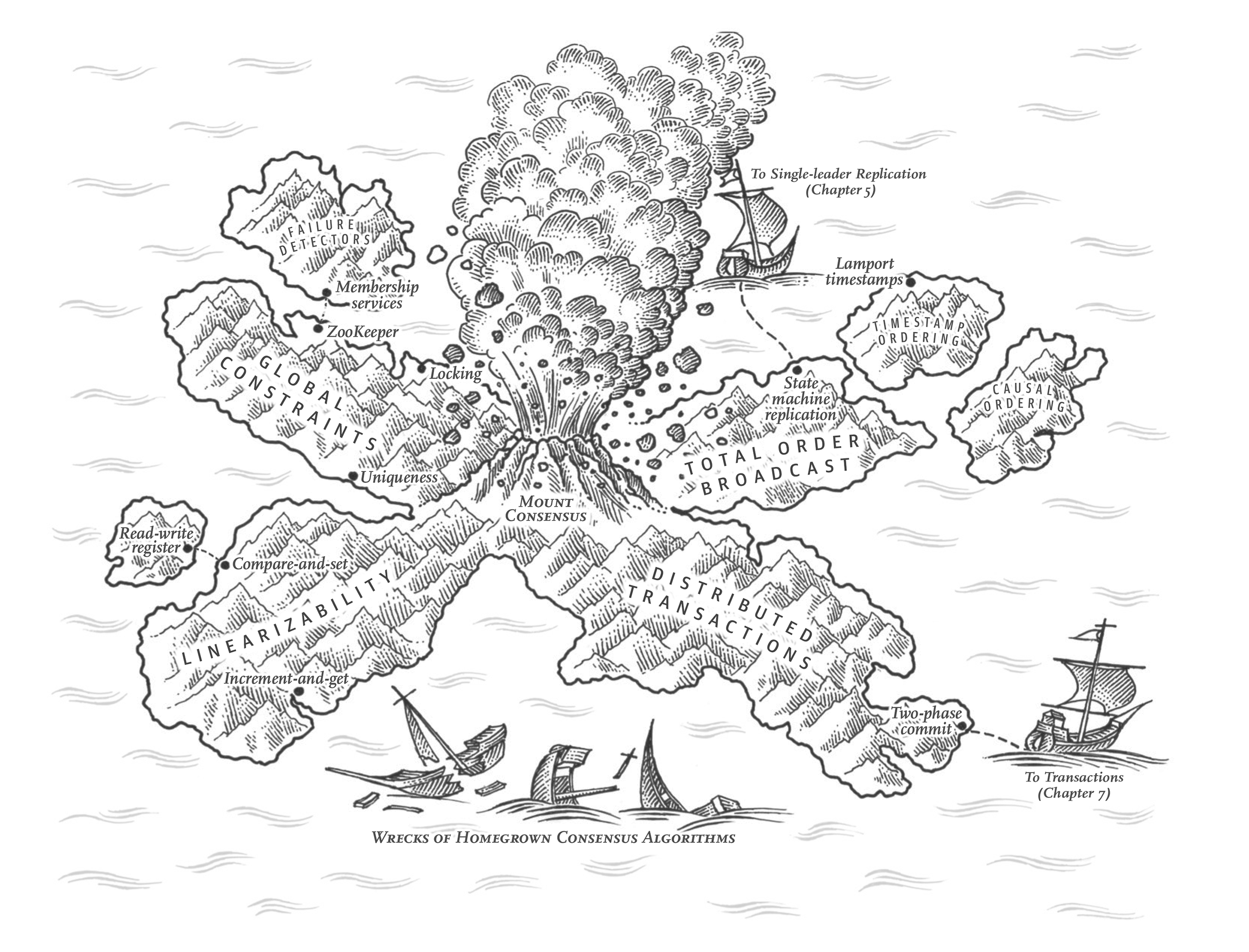
An ancient adage warns, “Never go to sea with two chronometers; take one or three.”

Frederick P. Brooks Jr., The Mythical Man-Month: Essays on Software Engineering (1995)

Lots of things can go wrong in distributed systems, as discussed in Chapter 9. If we want a service to continue working correctly despite those things going wrong, we need to find ways of tolerating faults.

One of the best tools we have for fault tolerance is replication. However, as we saw in Chapter 6, having multiple copies of the data on multiple replicas opens up the risk of inconsistencies. Reads might be handled by a replica that is not up-to-date, yielding stale results. If multiple replicas can accept writes, we have to deal with conflicts between values that were concurrently written on different replicas. At a high level, there are two competing philosophies for dealing with such issues:

Eventual consistency: In this philosophy, the fact that a system is replicated is made visible to the application, and you as application developer are expected to deal with the inconsistencies and conflicts that may arise. This approach is often used in systems with multi-leader (see “Multi-Leader Replication”) and leaderless replication (see “Leaderless Replication”).
Strong consistency: This philosophy says that applications should not have to worry about internal details of replication, and that the system should behave as if it was single-node. The advantage of this approach is that it’s simpler for you, the application developer. The disadvantage is that stronger consistency has a performance cost, and some kinds of fault that an eventually consistent system can tolerate cause outages in strongly consistent systems.

As always, which approach is better depends on your application. If you have an app where users can make changes to data while offline, then eventual consistency is inevitable, as discussed in “Sync Engines and Local-First Software”. However, eventual consistency can also be difficult for applications to deal with. If your replicas are located in datacenters with fast, reliable communication, then strong consistency is often appropriate because its cost is acceptable.

In this chapter we will dive deeper into the strongly consistent approach, looking at three areas:

One challenge is that “strong consistency” is quite vague, so we will develop a more precise definition of what we want to achieve: linearizability.
We will look at the problem of generating IDs and timestamps. This may sound unrelated to consistency but is actually closely connected.
We will explore how distributed systems can achieve linearizability while still remaining fault-tolerant; the answer is consensus algorithms.

Along the way, we will see that there are some fundamental limits on what is possible and what is not in a distributed system.

The topics of this chapter are notorious for being hard to implement correctly; it’s very easy to build systems that behave fine when there are no faults, but which completely fall apart when faced with an unlucky combination of faults that the designer of the system hadn’t considered. A lot of theory has been developed to help us think through those edge cases, which enables us to build systems that can robustly tolerate faults.

This chapter will only scratch the surface: we will stick with informal intuitions, and avoid the algorithmic nitty-gritty, formal models, and proofs. If you want to do serious work on consensus systems and similar infrastructure, you will need to go much deeper into the theory if you want any chance of your systems being robust. As usual, the literature references in this chapter provide some initial pointers.

Linearizability

If you want a replicated database to be as simple as possible to use, you should make it behave as if it wasn’t replicated at all. Then users don’t have to worry about replication lag, conflicts, and other inconsistencies. That would give us the advantage of fault tolerance, but without the complexity arising from having to think about multiple replicas.

This is the idea behind linearizability ¹ (also known as atomic consistency ², strong consistency, immediate consistency, or external consistency ³). The exact definition of linearizability is quite subtle, and we will explore it in the rest of this section. But the basic idea is to make a system appear as if there were only one copy of the data, and all operations on it are atomic. With this guarantee, even though there may be multiple replicas in reality, the application does not need to worry about them.

In a linearizable system, as soon as one client successfully completes a write, all clients reading from the database must be able to see the value just written. Maintaining the illusion of a single copy of the data means guaranteeing that the value read is the most recent, up-to-date value, and doesn’t come from a stale cache or replica. In other words, linearizability is a recency guarantee. To clarify this idea, let’s look at an example of a system that is not linearizable.

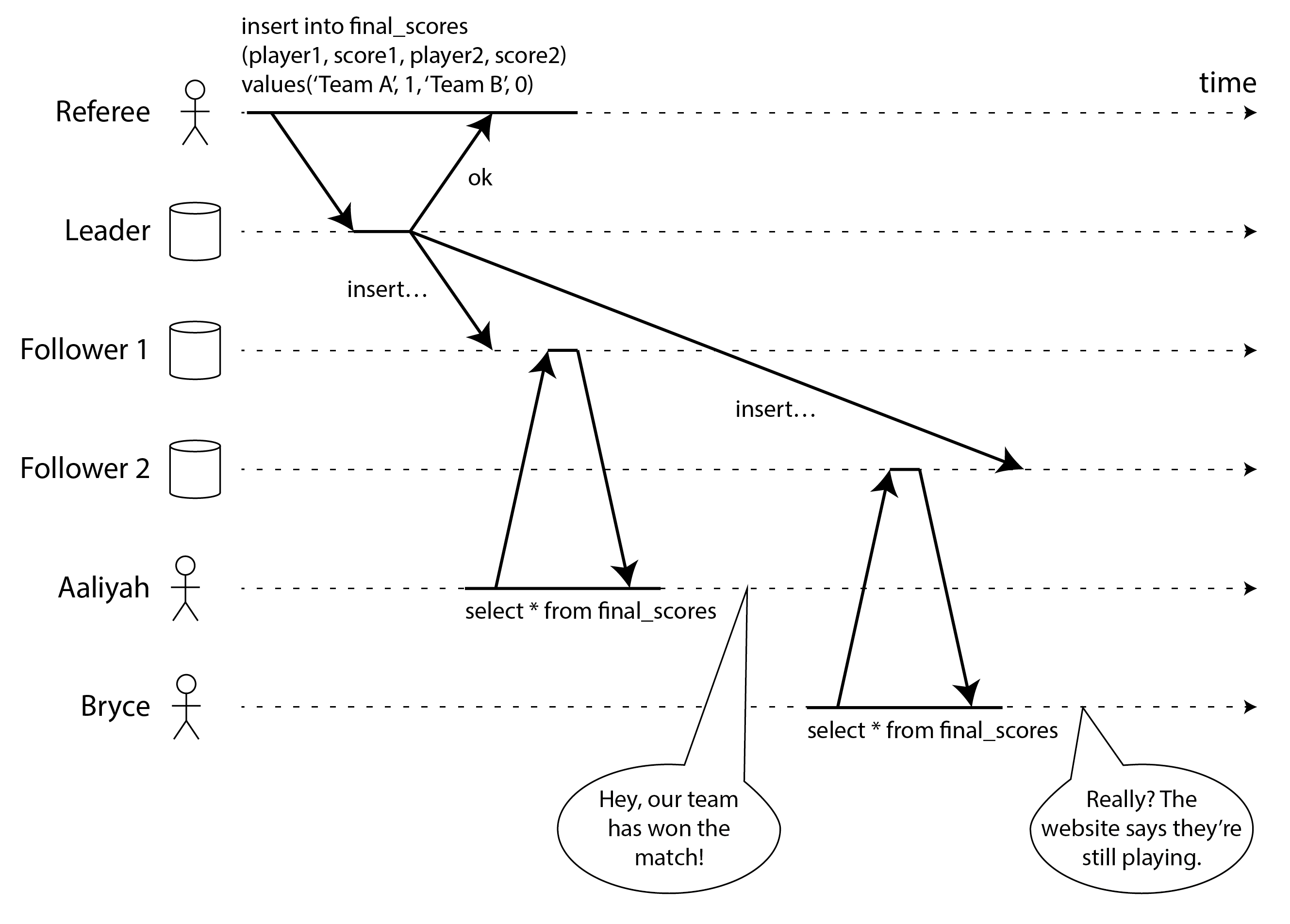
Figure 10-1 This system is not linearizable, causing sports fans to be confused.

Figure 10-1 shows an example of a nonlinearizable sports website ⁴. Aaliyah and Bryce are sitting in the same room, both checking their phones to see the outcome of a game their favorite team is playing. Just after the final score is announced, Aaliyah refreshes the page, sees the winner announced, and excitedly tells Bryce about it. Bryce incredulously hits reload on his own phone, but his request goes to a database replica that is lagging, and so his phone shows that the game is still ongoing.

If Aaliyah and Bryce had hit reload at the same time, it would have been less surprising if they had gotten two different query results, because they wouldn’t know at exactly what time their respective requests were processed by the server. However, Bryce knows that he hit the reload button (initiated his query) after he heard Aaliyah exclaim the final score, and therefore he expects his query result to be at least as recent as Aaliyah’s. The fact that his query returned a stale result is a violation of linearizability.

What Makes a System Linearizable?

In order to understand linearizability better, let’s look at some more examples. Figure 10-2 shows three clients concurrently reading and writing the same object x in a linearizable database. In distributed systems theory, x is called a register—in practice, it could be one key in a key-value store, one row in a relational database, or one document in a document database, for example.

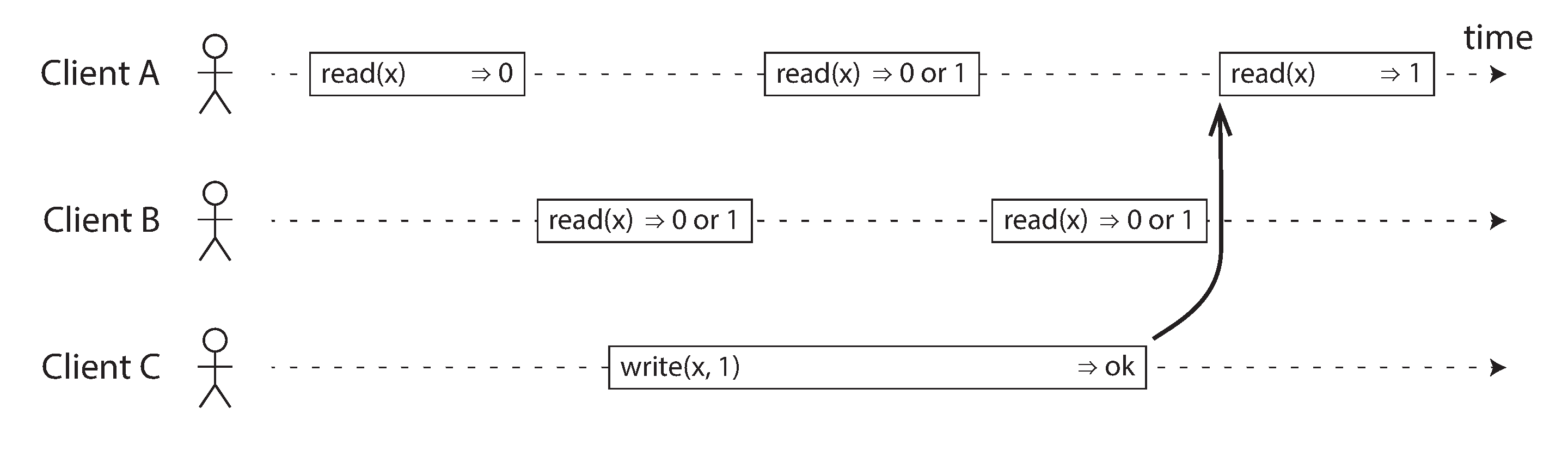
Figure 10-2 If a read request is concurrent with a write request, it may return either the old or the new value.

For simplicity, Figure 10-2 shows only the requests from the clients’ point of view, not the internals of the database. Each bar is a request made by a client, where the start of a bar is the time when the request was sent, and the end of a bar is when the response was received by the client. Due to variable network delays, a client doesn’t know exactly when the database processed its request—it only knows that it must have happened sometime between the client sending the request and receiving the response.

In this example, the register has two types of operations:

read(x) ⇒ v means the client requested to read the value of register x, and the database returned the value v.
write(x, v) ⇒ r means the client requested to set the register x to value v, and the database returned response r (which could be ok or error).

In Figure 10-2, the value of x is initially 0, and client C performs a write request to set it to 1. While this is happening, clients A and B are repeatedly polling the database to read the latest value. What are the possible responses that A and B might get for their read requests?

The first read operation by client A completes before the write begins, so it must definitely return the old value 0.
The last read by client A begins after the write has completed, so it must definitely return the new value 1 if the database is linearizable, because the read must have been processed after the write.
Any read operations that overlap in time with the write operation might return either 0 or 1, because we don’t know whether or not the write has taken effect at the time when the read operation is processed. These operations are concurrent with the write.

However, that is not yet sufficient to fully describe linearizability: if reads that are concurrent with a write can return either the old or the new value, then readers could see a value flip back and forth between the old and the new value several times while a write is going on. That is not what we expect of a system that emulates a “single copy of the data.”

To make the system linearizable, we need to add another constraint, illustrated in Figure 10-3.

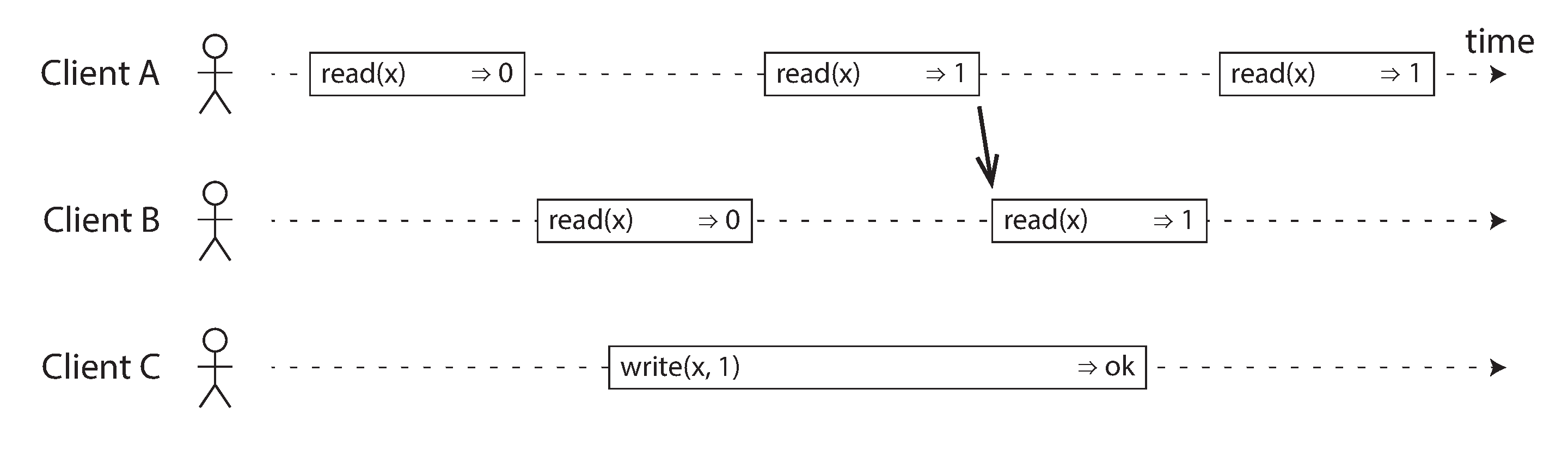
Figure 10-3 After any one read has returned the new value, all following reads (on the same or other clients) must also return the new value.

In a linearizable system we imagine that there must be some point in time (between the start and end of the write operation) at which the value of x atomically flips from 0 to 1. Thus, if one client’s read returns the new value 1, all subsequent reads must also return the new value, even if the write operation has not yet completed.

This timing dependency is illustrated with an arrow in Figure 10-3. Client A is the first to read the new value, 1. Just after A’s read returns, B begins a new read. Since B’s read occurs strictly after A’s read, it must also return 1, even though the write by C is still ongoing. (It’s the same situation as with Aaliyah and Bryce in Figure 10-1: after Aaliyah has read the new value, Bryce also expects to read the new value.)

We can further refine this timing diagram to visualize each operation taking effect atomically at some point in time ⁵, like in the more complex example shown in Figure 10-4. In this example we add a third type of operation besides read and write:

cas(x, vold, vnew) ⇒ r means the client requested an atomic compare-and-set operation (see “Conditional writes (compare-and-set)”). If the current value of the register x equals vold, it should be atomically set to vnew. If the value of x is different from vold, then the operation should leave the register unchanged and return an error. r is the database’s response (ok or error).

Each operation in Figure 10-4 is marked with a vertical line (inside the bar for each operation) at the time when we think the operation was executed. Those markers are joined up in a sequential order, and the result must be a valid sequence of reads and writes for a register (every read must return the value set by the most recent write).

The requirement of linearizability is that the lines joining up the operation markers always move forward in time (from left to right), never backward. This requirement ensures the recency guarantee we discussed earlier: once a new value has been written or read, all subsequent reads see the value that was written, until it is overwritten again.

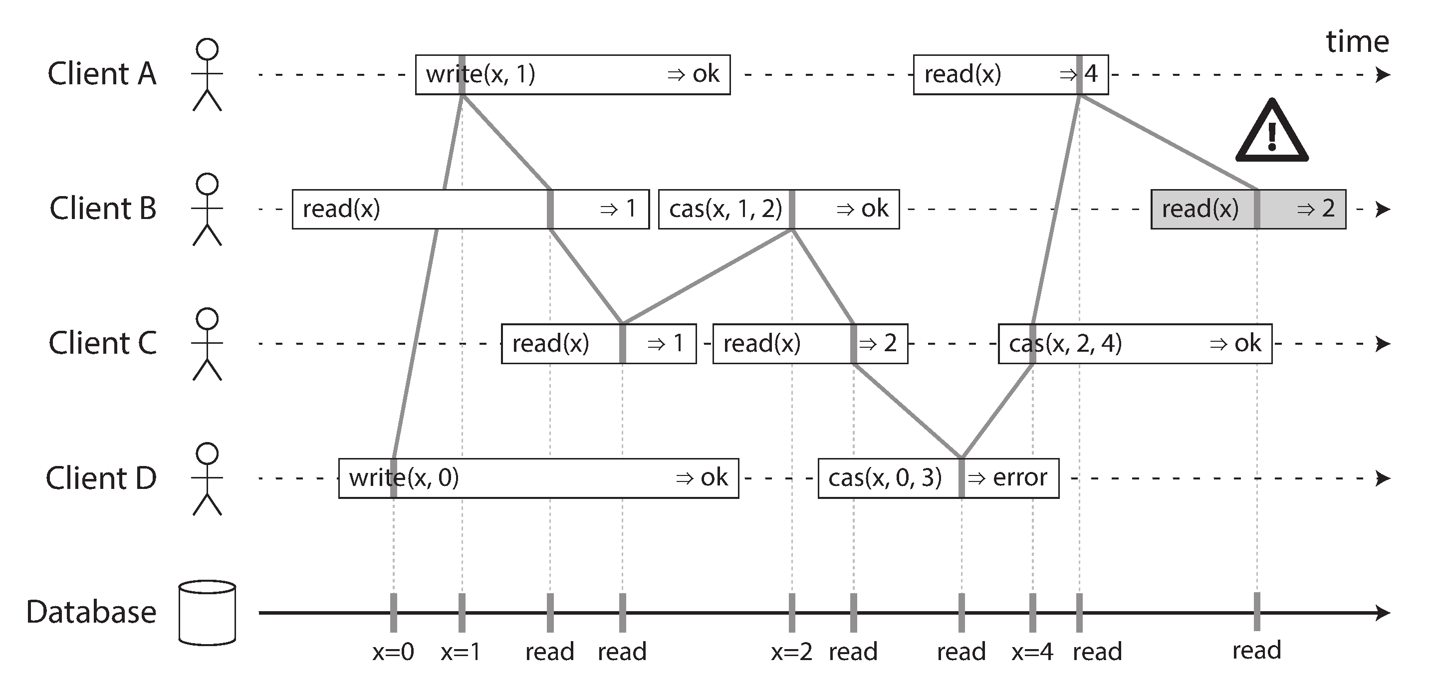
Figure 10-4 Visualizing the points in time at which the reads and writes appear to have taken effect. The final read by B is not linearizable.

There are a few interesting details to point out in Figure 10-4:

First client B sent a request to read x, then client D sent a request to set x to 0, and then client A sent a request to set x to 1. Nevertheless, the value returned to B’s read is 1 (the value written by A). This is okay: it means that the database first processed D’s write, then A’s write, and finally B’s read. Although this is not the order in which the requests were sent, it’s an acceptable order, because the three requests are concurrent. Perhaps B’s read request was slightly delayed in the network, so it only reached the database after the two writes.
Client B’s read returned 1 before client A received its response from the database, saying that the write of the value 1 was successful. This is also okay: it just means the ok response from the database to client A was slightly delayed in the network.
This model doesn’t assume any transaction isolation: another client may change a value at any time. For example, C first reads 1 and then reads 2, because the value was changed by B between the two reads. An atomic compare-and-set (cas) operation can be used to check the value hasn’t been concurrently changed by another client: B and C’s cas requests succeed, but D’s cas request fails (by the time the database processes it, the value of x is no longer 0).
The final read by client B (in a shaded bar) is not linearizable. The operation is concurrent with C’s cas write, which updates x from 2 to 4. In the absence of other requests, it would be okay for B’s read to return 2. However, client A has already read the new value 4 before B’s read started, so B is not allowed to read an older value than A. Again, it’s the same situation as with Aaliyah and Bryce in Figure 10-1.

That is the intuition behind linearizability; the formal definition ¹ describes it more precisely. It is possible (though computationally expensive) to test whether a system’s behavior is linearizable by recording the timings of all requests and responses, and checking whether they can be arranged into a valid sequential order ⁶ ⁷.

Just as there are various weak isolation levels for transactions besides serializability (see “Weak Isolation Levels”), there are also various weaker consistency models for replicated systems besides linearizability ⁸. In fact, the read-after-write, monotonic reads, and consistent prefix reads properties we saw in “Problems with Replication Lag” are examples of such weaker consistency models. Linearizability guarantees all these weaker properties, and more. In this chapter we will focus on linearizability, which is the strongest consistency model in common use.

LINEARIZABILITY VERSUS SERIALIZABILITY

Linearizability is easily confused with serializability (see “Serializability”), as both words seem to mean something like “can be arranged in a sequential order.” However, they are quite different guarantees, and it is important to distinguish between them:

Serializability: Serializability is an isolation property of transactions, where every transaction may read and write multiple objects (rows, documents, records). It guarantees that transactions behave the same as if they had executed in some serial order: that is, as if you first performed all of one transaction’s operations, then all of another transaction’s operations, and so on, without interleaving them. It is okay for that serial order to be different from the order in which the transactions were actually run ⁹.
Linearizability: Linearizability is a guarantee on reads and writes of a register (an individual object). It doesn’t group operations together into transactions, so it does not prevent problems such as write skew that involve multiple objects (see “Write Skew and Phantoms”). However, linearizability is a recency guarantee: it requires that if one operation finishes before another one starts, then the later operation must observe a state that is at least as new as the earlier operation. Serializability does not have that requirement: for example, stale reads are allowed by serializability ¹⁰.

(Sequential consistency is something else again ⁸, but we won’t discuss it here.)

A database may provide both serializability and linearizability, and this combination is known as strict serializability or strong one-copy serializability (strong-1SR) ¹¹ ¹². Single-node databases are typically linearizable. With distributed databases using optimistic methods like serializable snapshot isolation (see “Serializable Snapshot Isolation (SSI)”) the situation is more complicated: for example, CockroachDB provides serializability, and some recency guarantees on reads, but not strict serializability ¹³ because this would require expensive coordination between transactions ¹⁴.

It is also possible to combine a weaker isolation level with linearizability, or a weaker consistency model with serializability; in fact, consistency model and isolation level can be chosen largely independently from each other ¹⁵ ¹⁶.

Relying on Linearizability

In what circumstances is linearizability useful? Viewing the final score of a sporting match is perhaps a frivolous example: a result that is outdated by a few seconds is unlikely to cause any real harm in this situation. However, there a few areas in which linearizability is an important requirement for making a system work correctly.

Locking and leader election

A system that uses single-leader replication needs to ensure that there is indeed only one leader, not several (split brain). One way of electing a leader is to use a lease: every node that starts up tries to acquire the lease, and the one that succeeds becomes the leader ¹⁷. No matter how this mechanism is implemented, it must be linearizable: it should not be possible for two different nodes to acquire the lease at the same time.

Coordination services like Apache ZooKeeper ¹⁸ and etcd are often used to implement distributed leases and leader election. They use consensus algorithms to implement linearizable operations in a fault-tolerant way (we discuss such algorithms later in this chapter). There are still many subtle details to implementing leases and leader election correctly (see for example the fencing issue in “Distributed Locks and Leases”), and libraries like Apache Curator help by providing higher-level recipes on top of ZooKeeper. However, a linearizable storage service is the basic foundation for these coordination tasks.

Note

Strictly speaking, ZooKeeper provides linearizable writes, but reads may be stale, since there is no guarantee that they are served from the current leader ¹⁸. etcd since version 3 provides linearizable reads by default.

Distributed locking is also used at a much more granular level in some distributed databases, such as Oracle Real Application Clusters (RAC) ¹⁹. RAC uses a lock per disk page, with multiple nodes sharing access to the same disk storage system. Since these linearizable locks are on the critical path of transaction execution, RAC deployments usually have a dedicated cluster interconnect network for communication between database nodes.

Constraints and uniqueness guarantees

Uniqueness constraints are common in databases: for example, a username or email address must uniquely identify one user, and in a file storage service there cannot be two files with the same path and filename. If you want to enforce this constraint as the data is written (such that if two people try to concurrently create a user or a file with the same name, one of them will be returned an error), you need linearizability.

This situation is actually similar to a lock: when a user registers for your service, you can think of them acquiring a “lock” on their chosen username. The operation is also very similar to an atomic compare-and-set, setting the username to the ID of the user who claimed it, provided that the username is not already taken.

Similar issues arise if you want to ensure that a bank account balance never goes negative, or that you don’t sell more items than you have in stock in the warehouse, or that two people don’t concurrently book the same seat on a flight or in a theater. These constraints all require there to be a single up-to-date value (the account balance, the stock level, the seat occupancy) that all nodes agree on.

In real applications, it is sometimes acceptable to treat such constraints loosely (for example, if a flight is overbooked, you can move customers to a different flight and offer them compensation for the inconvenience). In such cases, linearizability may not be needed, and we will discuss such loosely interpreted constraints in “Timeliness and Integrity”.

However, a hard uniqueness constraint, such as the one you typically find in relational databases, requires linearizability. Other kinds of constraints, such as foreign key or attribute constraints, can be implemented without linearizability ²⁰.

Cross-channel timing dependencies

Notice a detail in Figure 10-1: if Aaliyah hadn’t exclaimed the score, Bryce wouldn’t have known that the result of his query was stale. He would have just refreshed the page again a few seconds later, and eventually seen the final score. The linearizability violation was only noticed because there was an additional communication channel in the system (Aaliyah’s voice to Bryce’s ears).

Similar situations can arise in computer systems. For example, say you have a website where users can upload a video, and a background process transcodes the video to a lower quality that can be streamed on slow internet connections. The architecture and dataflow of this system is illustrated in Figure 10-5.

The video transcoder needs to be explicitly instructed to perform a transcoding job, and this instruction is sent from the web server to the transcoder via a message queue (see “Messaging Systems”). The web server doesn’t place the entire video on the queue, since most message brokers are designed for small messages, and a video may be many megabytes in size. Instead, the video is first written to a file storage service, and once the write is complete, the instruction to the transcoder is placed on the queue.

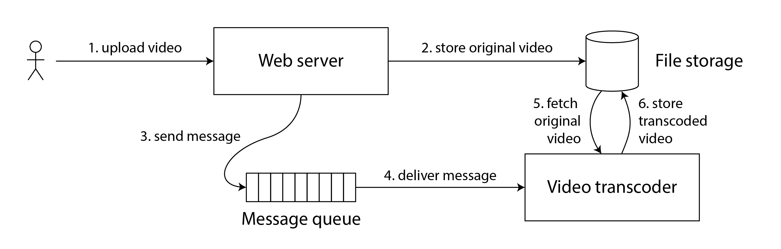
Figure 10-5 The web server and video transcoder communicate both through file storage and a message queue, opening the potential for race conditions.

If the file storage service is linearizable, then this system should work fine. If it is not linearizable, there is the risk of a race condition: the message queue (steps 3 and 4 in Figure 10-5) might be faster than the internal replication inside the storage service. In this case, when the transcoder fetches the original video (step 5), it might see an old version of the file, or nothing at all. If it processes an old version of the video, the original and transcoded videos in the file storage become permanently inconsistent with each other.

This problem arises because there are two different communication channels between the web server and the transcoder: the file storage and the message queue. Without the recency guarantee of linearizability, race conditions between these two channels are possible. This situation is analogous to Figure 10-1, where there was also a race condition between two communication channels: the database replication and the real-life audio channel between Aaliyah’s mouth and Bryce’s ears.

A similar race condition occurs if you have a mobile app that can receive push notifications, and the app fetches some data from a server when it receives a push notification. If the data fetch might go to a lagging replica, it could happen that the push notification goes through quickly, but the subsequent fetch doesn’t see the data that the push notification was about.

Linearizability is not the only way of avoiding this race condition, but it’s the simplest to understand. If you control the additional communication channel (like in the case of the message queue, but not in the case of Aaliyah and Bryce), you can use alternative approaches similar to what we discussed in “Reading Your Own Writes”, at the cost of additional complexity.

Implementing Linearizable Systems

Now that we’ve looked at a few examples in which linearizability is useful, let’s think about how we might implement a system that offers linearizable semantics.

Since linearizability essentially means “behave as though there is only a single copy of the data, and all operations on it are atomic,” the simplest answer would be to really only use a single copy of the data. However, that approach would not be able to tolerate faults: if the node holding that one copy failed, the data would be lost, or at least inaccessible until the node was brought up again.

Let’s revisit the replication methods from Chapter 6, and compare whether they can be made linearizable:

Single-leader replication (potentially linearizable): In a system with single-leader replication, the leader has the primary copy of the data that is used for writes, and the followers maintain backup copies of the data on other nodes. As long as you perform all reads and writes on the leader, they are likely to be linearizable. However, this assumes that you know for sure who the leader is. As discussed in “Distributed Locks and Leases”, it is quite possible for a node to think that it is the leader, when in fact it is not—and if the delusional leader continues to serve requests, it is likely to violate linearizability ²¹. With asynchronous replication, failover may even lose committed writes, which violates both durability and linearizability.

Sharding a single-leader database, with a separate leader per shard, does not affect linearizability, since it is only a single-object guarantee. Cross-shard transactions are a different matter (see “Distributed Transactions”).

Consensus algorithms (likely linearizable): Some consensus algorithms are essentially single-leader replication with automatic leader election and failover. They are carefully designed to prevent split brain, allowing them to implement linearizable storage safely. ZooKeeper uses the Zab consensus algorithm ²² and etcd uses Raft ²³, for example. However, just because a system uses consensus does not guarantee that all operations on it are linearizable: if it allows reads on a node without checking that it is still the leader, the results of the read may be stale if a new leader has just been elected.
Multi-leader replication (not linearizable): Systems with multi-leader replication are generally not linearizable, because they concurrently process writes on multiple nodes and asynchronously replicate them to other nodes. For this reason, they can produce conflicting writes that require resolution (see “Dealing with Conflicting Writes”).
Leaderless replication (probably not linearizable): For systems with leaderless replication (Dynamo-style; see “Leaderless Replication”), people sometimes claim that you can obtain “strong consistency” by requiring quorum reads and writes (w + r > n). Depending on the exact algorithm, and depending on how you define strong consistency, this is not quite true.

“Last write wins” conflict resolution methods based on time-of-day clocks (e.g., in Cassandra and ScyllaDB) are almost certainly nonlinearizable, because clock timestamps cannot be guaranteed to be consistent with actual event ordering due to clock skew (see “Relying on Synchronized Clocks”). Even with quorums, nonlinearizable behavior is possible, as demonstrated in the next section.

Linearizability and quorums

Intuitively, it seems as though quorum reads and writes should be linearizable in a Dynamo-style model. However, when we have variable network delays, it is possible to have race conditions, as demonstrated in Figure 10-6.

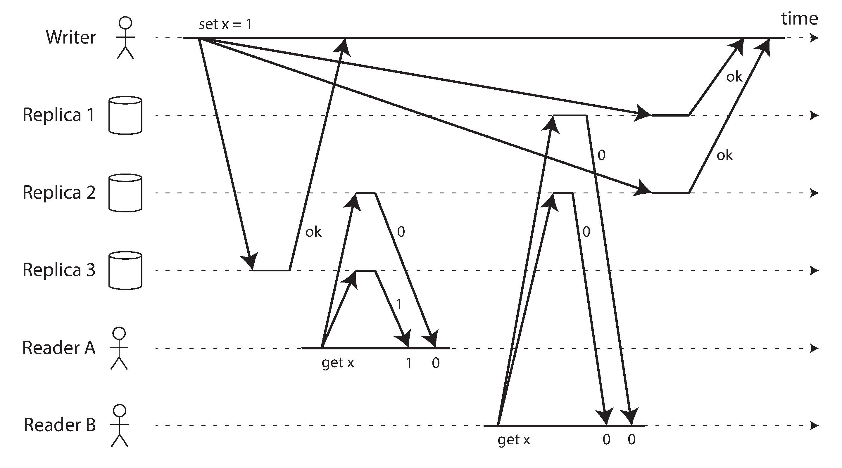
Figure 10-6 Quorums are not sufficient to ensure linearizability if network delays are variable.

In Figure 10-6, the initial value of x is 0, and a writer client is updating x to 1 by sending the write to all three replicas (n = 3, w = 3). Concurrently, client A reads from a quorum of two nodes (r = 2) and sees the new value 1 on one of the nodes. Also concurrently with the write, client B reads from a different quorum of two nodes, and gets back the old value 0 from both.

The quorum condition is met (w + r > n), but this execution is nevertheless not linearizable: B’s request begins after A’s request completes, but B returns the old value while A returns the new value. (It’s once again the Aaliyah and Bryce situation from Figure 10-1.)

It is possible to make Dynamo-style quorums linearizable at the cost of reduced performance: a reader must perform read repair (see “Catching up on missed writes”) synchronously, before returning results to the application ²⁴. Moreover, before writing, a writer must read the latest state of a quorum of nodes to fetch the latest timestamp of any prior write, and ensure that the new write has a greater timestamp ²⁵ ²⁶. However, Riak does not perform synchronous read repair due to the performance penalty. Cassandra does wait for read repair to complete on quorum reads ²⁷, but it loses linearizability due to its use of time-of-day clocks for timestamps.

Moreover, only linearizable read and write operations can be implemented in this way; a linearizable compare-and-set operation cannot, because it requires a consensus algorithm ²⁸.

In summary, it is safest to assume that a leaderless system with Dynamo-style replication does not provide linearizability, even with quorum reads and writes.

The Cost of Linearizability

As some replication methods can provide linearizability and others cannot, it is interesting to explore the pros and cons of linearizability in more depth.

We already discussed some use cases for different replication methods in Chapter 6; for example, we saw that multi-leader replication is often a good choice for multi-region replication (see “Geographically Distributed Operation”). An example of such a deployment is illustrated in Figure 10-7.

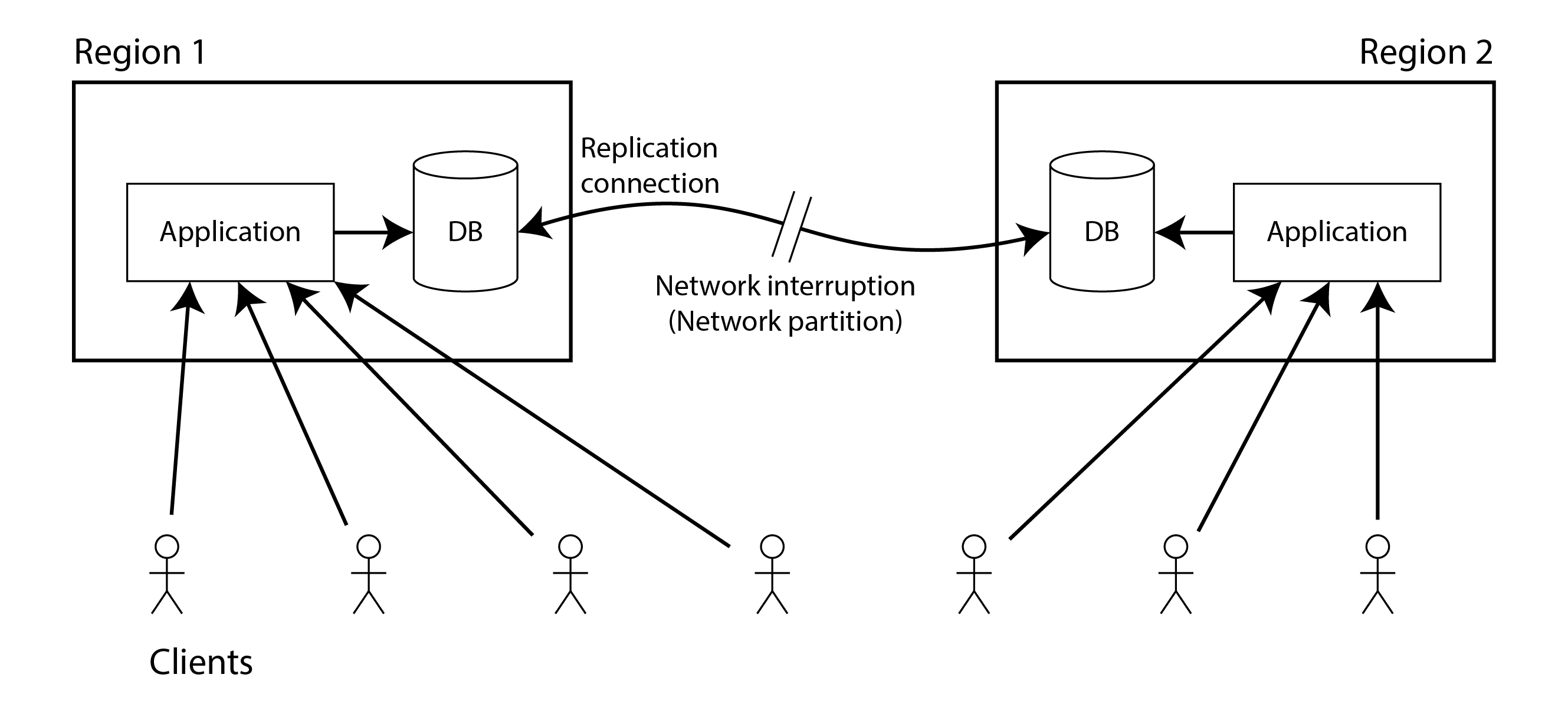
Figure 10-7 A network interruption forcing a choice between linearizability and availability.

Consider what happens if there is a network interruption between the two regions. Let’s assume that the network within each region is working, and clients can reach their local region, but the regions cannot connect to each other. This is known as a network partition.

With a multi-leader database, each region can continue operating normally: since writes from one region are asynchronously replicated to the other, the writes are simply queued up and exchanged when network connectivity is restored.

On the other hand, if single-leader replication is used, then the leader must be in one of the regions. Any writes and any linearizable reads must be sent to the leader—thus, for any clients connected to a follower region, those read and write requests must be sent synchronously over the network to the leader region.

If the network between regions is interrupted in a single-leader setup, clients connected to follower regions cannot contact the leader, so they cannot make any writes to the database, nor any linearizable reads. They can still make reads from the follower, but they might be stale (nonlinearizable). If the application requires linearizable reads and writes, the network interruption causes the application to become unavailable in the regions that cannot contact the leader.

If clients can connect directly to the leader region, this is not a problem, since the application continues to work normally there. But clients that can only reach a follower region will experience an outage until the network link is repaired.

The CAP theorem

This issue is not just a consequence of single-leader and multi-leader replication: any linearizable database has this problem, no matter how it is implemented. The issue also isn’t specific to multi-region deployments, but can occur on any unreliable network, even within one region. The trade-off is as follows:

If your application requires linearizability, and some replicas are disconnected from the other replicas due to a network problem, then some replicas cannot process requests while they are disconnected: they must either wait until the network problem is fixed, or return an error (either way, they become unavailable). This choice is sometimes known as CP (consistent under network partitions).
If your application does not require linearizability, then it can be written in a way that each replica can process requests independently, even if it is disconnected from other replicas (e.g., multi-leader). In this case, the application can remain available in the face of a network problem, but its behavior is not linearizable. This choice is known as AP (available under network partitions).

Thus, applications that don’t require linearizability can be more tolerant of network problems. This insight is popularly known as the CAP theorem ²⁹ ³⁰ ³¹ ³², named by Eric Brewer in 2000, although the trade-off had been known to designers of distributed databases since the 1970s ³³ ³⁴ ³⁵.

CAP was originally proposed as a rule of thumb, without precise definitions, with the goal of starting a discussion about trade-offs in databases. At the time, many distributed databases focused on providing linearizable semantics on a cluster of machines with shared storage ¹⁹, and CAP encouraged database engineers to explore a wider design space of distributed shared-nothing systems, which were more suitable for implementing large-scale web services ³⁶. CAP deserves credit for this culture shift—it helped trigger the NoSQL movement, a burst of new database technologies around the mid-2000s.

THE UNHELPFUL CAP THEOREM

CAP is sometimes presented as Consistency, Availability, Partition tolerance: pick 2 out of 3. Unfortunately, putting it this way is misleading ³² because network partitions are a kind of fault, so they aren’t something about which you have a choice: they will happen whether you like it or not.

At times when the network is working correctly, a system can provide both consistency (linearizability) and total availability. When a network fault occurs, you have to choose between either linearizability or total availability. Thus, a better way of phrasing CAP would be either Consistent or Available when Partitioned ³⁷. A more reliable network needs to make this choice less often, but at some point the choice is inevitable.

The CP/AP classification scheme has several further flaws ⁴. Consistency is formalized as linearizability (the theorem doesn’t say anything about weaker consistency models), and the formalization of availability ³⁰ does not match the usual meaning of the term ³⁸. Many highly available (fault-tolerant) systems actually do not meet CAP’s idiosyncratic definition of availability. Moreover, some system designers choose (with good reason) to provide neither linearizability nor the form of availability that the CAP theorem assumes, so those systems are neither CP nor AP ³⁹ ⁴⁰.

All in all, there is a lot of misunderstanding and confusion around CAP, and it does not help us understand systems better, so CAP is best avoided.

The CAP theorem as formally defined ³⁰ is of very narrow scope: it only considers one consistency model (namely linearizability) and one kind of fault (network partitions, which according to data from Google are the cause of less than 8% of incidents ⁴¹). It doesn’t say anything about network delays, dead nodes, or other trade-offs. Thus, although CAP has been historically influential, it has little practical value for designing systems ⁴ ³⁸.

There have been efforts to generalize CAP. For example, the PACELC principle observes that system designers might also choose to weaken consistency at times when the network is working fine in order to reduce latency ³⁹ ⁴⁰ ⁴². Thus, during a network partition (P), we need to choose between availability (A) and consistency (C); else (E), when there is no partition, we may choose between low latency (L) and consistency (C). However, this definition inherits several problems with CAP, such as the counterintuitive definitions of consistency and availability.

There are many more interesting impossibility results in distributed systems ⁴³, and CAP has now been superseded by more precise results ⁴⁴ ⁴⁵, so it is of mostly historical interest today.

Linearizability and network delays

Although linearizability is a useful guarantee, surprisingly few systems are actually linearizable in practice. For example, even RAM on a modern multi-core CPU is not linearizable ⁴⁶: if a thread running on one CPU core writes to a memory address, and a thread on another CPU core reads the same address shortly afterward, it is not guaranteed to read the value written by the first thread (unless a memory barrier or fence ⁴⁷ is used).

The reason for this behavior is that every CPU core has its own memory cache and store buffer. Memory access first goes to the cache by default, and any changes are asynchronously written out to main memory. Since accessing data in the cache is much faster than going to main memory ⁴⁸, this feature is essential for good performance on modern CPUs. However, there are now several copies of the data (one in main memory, and perhaps several more in various caches), and these copies are asynchronously updated, so linearizability is lost.

Why make this trade-off? It makes no sense to use the CAP theorem to justify the multi-core memory consistency model: within one computer we usually assume reliable communication, and we don’t expect one CPU core to be able to continue operating normally if it is disconnected from the rest of the computer. The reason for dropping linearizability is performance, not fault tolerance ³⁹.

The same is true of many distributed databases that choose not to provide linearizable guarantees: they do so primarily to increase performance, not so much for fault tolerance ⁴². Linearizability is slow—and this is true all the time, not only during a network fault.

Can’t we maybe find a more efficient implementation of linearizable storage? It seems the answer is no: Attiya and Welch ⁴⁹ prove that if you want linearizability, the response time of read and write requests is at least proportional to the uncertainty of delays in the network. In a network with highly variable delays, like most computer networks (see “Timeouts and Unbounded Delays”), the response time of linearizable reads and writes is inevitably going to be high. A faster algorithm for linearizability does not exist, but weaker consistency models can be much faster, so this trade-off is important for latency-sensitive systems. In “Timeliness and Integrity” we will discuss some approaches for avoiding linearizability without sacrificing correctness.

ID Generators and Logical Clocks

In many applications you need to assign some sort of unique ID to database records when they are created, which gives you a primary key by which you can refer to those records. In single-node databases it is common to use an auto-incrementing integer, which has the advantage that it can be stored in only 64 bits (or even 32 bits if you are sure that you will never have more than 4 billion records, but that is risky).

Another advantage of such auto-incrementing IDs is that the order of the IDs tells you the order in which the records were created. For example, Figure 10-8 shows a chat application that assigns auto-incrementing IDs to chat messages as they are posted. You can then display the messages in order of increasing ID, and the resulting chat threads will make sense: Aaliyah posts a question that is assigned ID 1, and Bryce’s answer to the question is assigned a greater ID, namely 3.

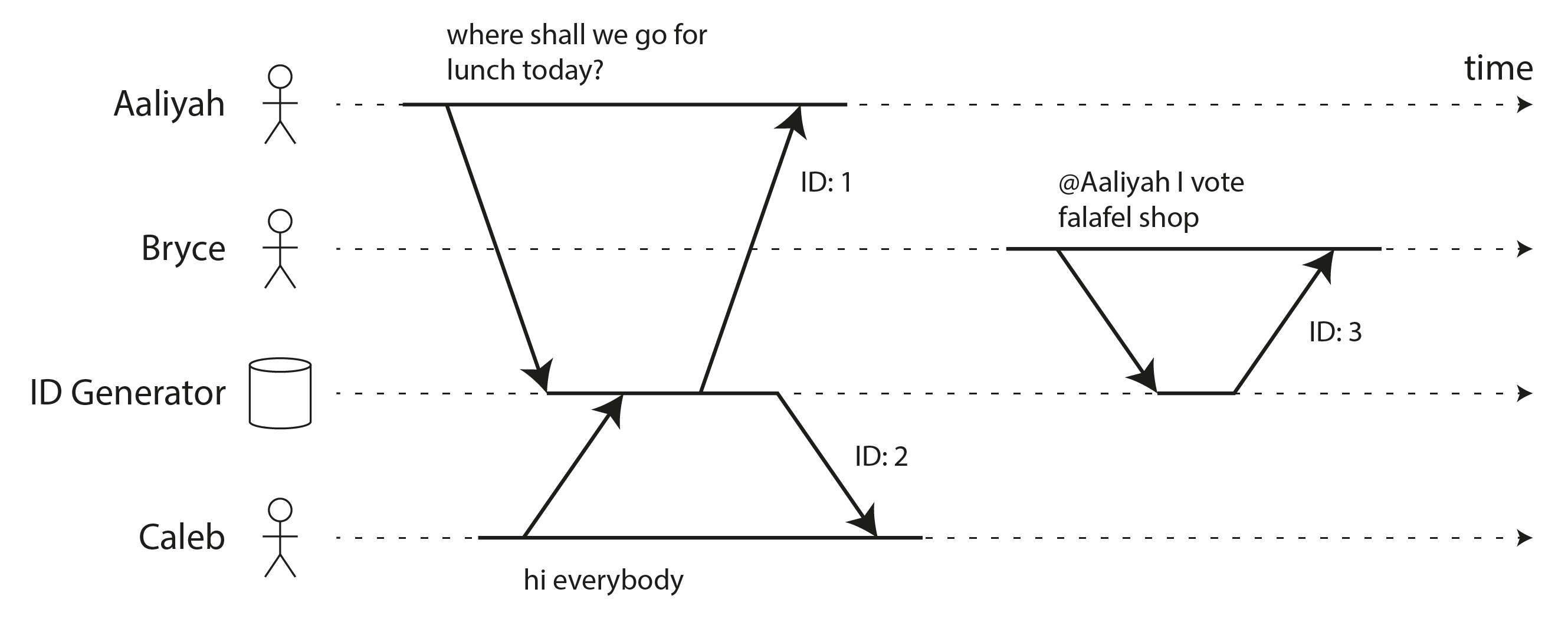
Figure 10-8 An ID generator that assigns auto-incrementing integer IDs to messages in a chat application.

This single-node ID generator is another example of a linearizable system. Each request to fetch the ID is an operation that atomically increments a counter and returns the old counter value (a fetch-and-add operation); linearizability ensures that if the posting of Aaliyah’s message completes before Bryce’s posting begins, then Bryce’s ID must be greater than Aaliyah’s. The messages by Aaliyah and Caleb in Figure 10-8 are concurrent, so linearizability doesn’t specify how their IDs must be ordered, as long as they are unique.

An in-memory single-node ID generator is easy to implement: you can use the atomic increment instruction provided by your CPU, which allows multiple threads to safely increment the same counter. It’s a bit more effort to make the counter persistent, so that the node can crash and restart without resetting the counter value, which would result in duplicate IDs. But the real problems are:

A single-node ID generator is not fault-tolerant because that node is a single point of failure.
It’s slow if you want to create a record in another region, as you potentially have to make a round-trip to the other side of the planet just to get an ID.
That single node could become a bottleneck if you have high write throughput.

There are various alternative options for ID generators that you can consider:

Sharded ID assignment: You could have multiple nodes that assign IDs—for example, one that generates only even numbers, and one that generates only odd numbers. In general, you can reserve some bits in the ID to contain a shard number. Those IDs are still compact, but you lose the ordering property: for example, if you have chat messages with IDs 16 and 17, you don’t know whether message 16 was actually sent first, because the IDs were assigned by different nodes, and one node might have been ahead of the other.
Preallocated blocks of IDs: Instead of requesting individual IDs from the single-node ID generator, it could hand out blocks of IDs. For example, node A might claim the block of IDs from 1 to 1,000, and node B might claim the block from 1,001 to 2,000. Then each node can independently hand out IDs from its block, and request a new block from the single-node ID generator when its supply of sequence numbers begins to run low. However, this scheme doesn’t ensure correct ordering either: it could happen that one message is given an ID in the range from 1,001 to 2,000, and a later message is given an ID in the range from 1 to 1,000 if the ID was assigned by a different node.
Random UUIDs: You can use universally unique identifiers (UUIDs), also known as globally unique identifiers (GUIDs). These have the big advantage that they can be generated locally on any node without requiring communication, but they require more space (128 bits). There are several different versions of UUIDs; the simplest is version 4, which is essentially a random number that is so long that is very unlikely that two nodes would ever pick the same one. Unfortunately, the order of such IDs is also random, so comparing two IDs tells you nothing about which one is newer.
Wall-clock timestamp made unique: If your nodes’ time-of-day clock is kept approximately correct using NTP, you can generate IDs by putting a timestamp from that clock in the most significant bits, and filling the remaining bits with extra information that ensures the ID is unique even if the timestamp is not—for example, a shard number and a per-shard incrementing sequence number, or a long random value. This approach is used in Version 7 UUIDs ⁵⁰, Twitter’s Snowflake ⁵¹, ULIDs ⁵², Hazelcast’s Flake ID generator, MongoDB ObjectIDs, and many similar schemes ⁵⁰. You can implement these ID generators in application code or within a database ⁵³.

All these schemes generate IDs that are unique (at least with high enough probability that collisions are vanishingly rare), but they have much weaker ordering guarantees for IDs than the single-node auto-incrementing scheme.

As discussed in “Timestamps for ordering events”, wall-clock timestamps can provide at best an approximate ordering: if an earlier write gets a timestamp from a slightly fast clock, and a later write’s timestamp is from a slightly slow clock, the timestamp order may be inconsistent with the order in which the events actually happened. With clock jumps due to using a non-monotonic clock, even the timestamps generated by a single node might be ordered incorrectly. ID generators based on wall-clock time are therefore unlikely to be linearizable.

You can reduce such ordering inconsistencies by relying on high-precision clock synchronization, using atomic clocks or GPS receivers. But it would also be nice to be able to generate IDs that are unique and correctly ordered without relying on special hardware. That’s what logical clocks are about.

Logical Clocks

In “Unreliable Clocks” we discussed time-of-day clocks and monotonic clocks. Both of these are physical clocks: they measure the passing of seconds (or milliseconds, microseconds, etc.).

In distributed systems it is common to also use another kind of clock, called a logical clock. While a physical clock is a hardware device that counts the seconds that have elapsed, a logical clock is an algorithm that counts the events that have occurred. A timestamp from a logical clock therefore doesn’t tell you what time it is, but you can compare two timestamps from a logical clock to tell which one is earlier and which one is later.

The requirements for a logical clock are typically:

that its timestamps are compact (a few bytes in size) and unique;
that you can compare any two timestamps (i.e. they are totally ordered); and
that the order of timestamps is consistent with causality: if operation A happened before B, then A’s timestamp is less than B’s timestamp. (We discussed causality previously in “The “happens-before” relation and concurrency”.)

A single-node ID generator meets these requirements, but the distributed ID generators we just discussed do not meet the causal ordering requirement.

Lamport timestamps

Fortunately, there is a simple method for generating logical timestamps that is consistent with causality, and which you can use as a distributed ID generator. It is called a Lamport clock, proposed in 1978 by Leslie Lamport ⁵⁴, in what is now one of the most-cited papers in the field of distributed systems.

Figure 10-9 shows how a Lamport clock would work in the chat example of Figure 10-8. Each node has a unique identifier, which in Figure 10-9 is the name “Aaliyah”, “Bryce”, or “Caleb”, but which in practice could be a random UUID or something similar. Moreover, each node keeps a counter of the number of operations it has processed. A Lamport timestamp is then simply a pair of (counter, node ID). Two nodes may sometimes have the same counter value, but by including the node ID in the timestamp, each timestamp is made unique.

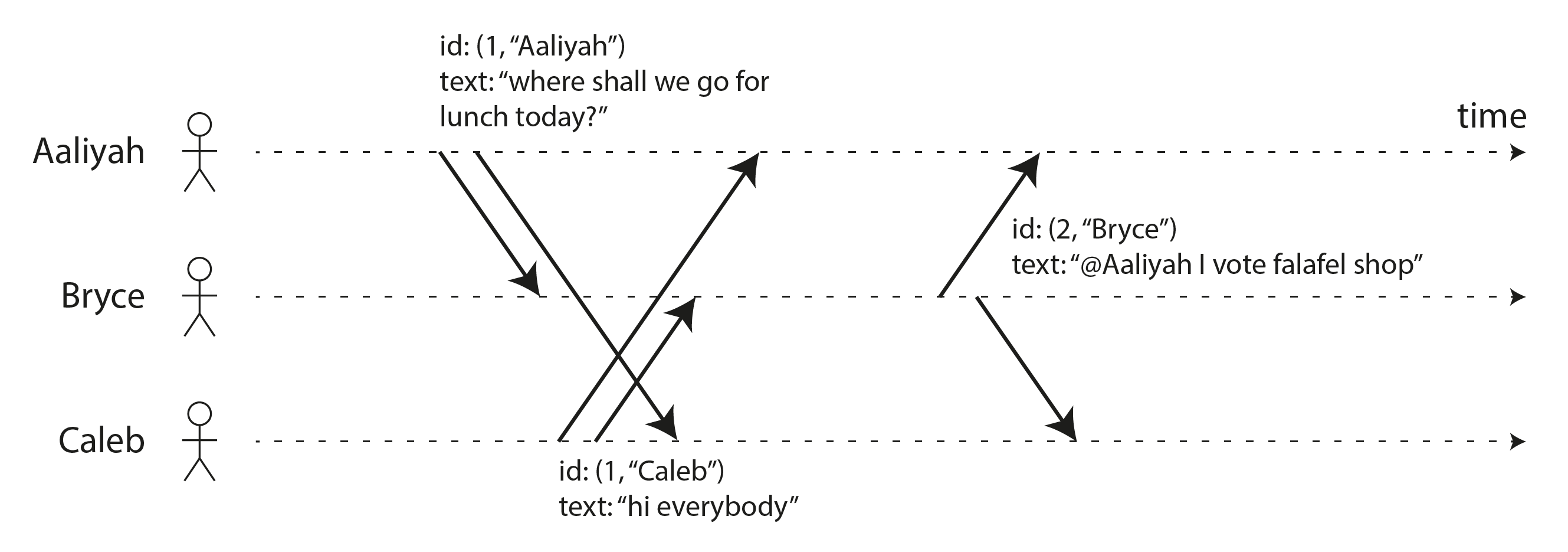
Figure 10-9 Lamport timestamps provide a total ordering consistent with causality.

Every time a node generates a timestamp, it increments its counter value and uses the new value. Moreover, every time a node sees a timestamp from another node, if the counter value in that timestamp is greater than its local counter value, it increases its local counter to match the value in the timestamp.

In Figure 10-9, Aaliyah had not yet seen Caleb’s message when posting her own, and vice versa. Assuming both users start with an initial counter value of 0, both therefore increment their local counter and attach the new counter value of 1 to their message. When Bryce receives those messages, he increases his local counter value to 1. Finally, Bryce sends a reply to Aaliyah’s message, for which he increments his local counter and attaches the new value of 2 to the message.

To compare two Lamport timestamps, we first compare their counter value: for example, (2, “Bryce”) is greater than (1, “Aaliyah”) and also greater than (1, “Caleb”). If two timestamps have the same counter, we compare their node IDs instead, using the usual lexicographic string comparison. Thus, the timestamp order in this example is (1, “Aaliyah”) < (1, “Caleb”) < (2, “Bryce”).

Hybrid logical clocks

Lamport timestamps are good at capturing the order in which things happened, but they have some limitations:

Since they have no direct relation to physical time, you can’t use them to find, say, all the messages that were posted on a particular date—you would need to store the physical time separately.
If two nodes never communicate, one node’s counter increments will never be reflected in the other one’s counter. As a result, it could happen that events generated around the same time on different nodes have wildly different counter values.

A hybrid logical clock combines the advantages of physical time-of-day clocks with the ordering guarantees of Lamport clocks ⁵⁵. Like a physical clock, it counts seconds or microseconds. Like a Lamport clock, when one node sees a timestamp from another node that is greater than its local clock value, it moves its own local value forward to match the other node’s timestamp. As a result, if one node’s clock is running fast, the other nodes will similarly move their clocks forward when they communicate.

Every time a timestamp from a hybrid logical clock is generated, it is also incremented, which ensures that the clock monotonically moves forward, even if the underlying physical clock jumps backwards, for example due to NTP adjustments. Thus, the hybrid logical clock might be slightly ahead of the underlying physical clock. Details of the algorithm ensure that this discrepancy remains as small as possible.

As a result, you can treat a timestamp from a hybrid logical clock almost like a timestamp from a conventional time-of-day clock, with the added property that its ordering is consistent with the happens-before relation. It doesn’t depend on any special hardware, and requires only roughly synchronized clocks. Hybrid logical clocks are used by CockroachDB, for example.

Lamport/hybrid logical clocks vs. vector clocks

In “Multi-version concurrency control (MVCC)” we discussed how snapshot isolation is often implemented: essentially, by giving each transaction a transaction ID, and allowing each transaction to see writes made by transactions with a lower ID, but to make writes by transactions with higher IDs invisible. Lamport clocks and hybrid logical clocks are a good way of generating these transaction IDs, because they ensure that the snapshot is consistent with causality ⁵⁶.

When multiple timestamps are generated concurrently, these algorithms order them arbitrarily. This means that when you look at two timestamps, you generally can’t tell whether they were generated concurrently or whether one happened before the other. (In the example of Figure 10-9 you actually can tell that Aaliyah and Caleb’s messages must have been concurrent, because they have the same counter value, but when the counter values are different you can’t tell whether they were concurrent.)

If you want to be able to determine when records were created concurrently, you need a different algorithm, such as a vector clock. The downside is that the timestamps from a vector clock are much bigger—potentially one integer for every node in the system. See “Detecting Concurrent Writes” for more details on detecting concurrency.

Linearizable ID Generators

Although Lamport clocks and hybrid logical clocks provide useful ordering guarantees, that ordering is still weaker than the linearizable single-node ID generator we talked about previously. Recall that linearizability requires that if request A completed before request B began, then B must have the higher ID, even if A and B never communicated with each other. On the other hand, Lamport clocks can only ensure that a node generates timestamps that are greater than any other timestamp that node has seen, but it can’t say anything about timestamps that it hasn’t seen.

Figure 10-10 shows how a non-linearizable ID generator could cause problems. Imagine a social media website where user A wants to share an embarrassing photo privately with their friends. A’s account is initially public, but using their laptop, A first changes their account settings to private. Then A uses their phone to upload the photo. Since A performed these updates in sequence, they might reasonably expect the photo upload to be subject to the new, restricted account permissions.

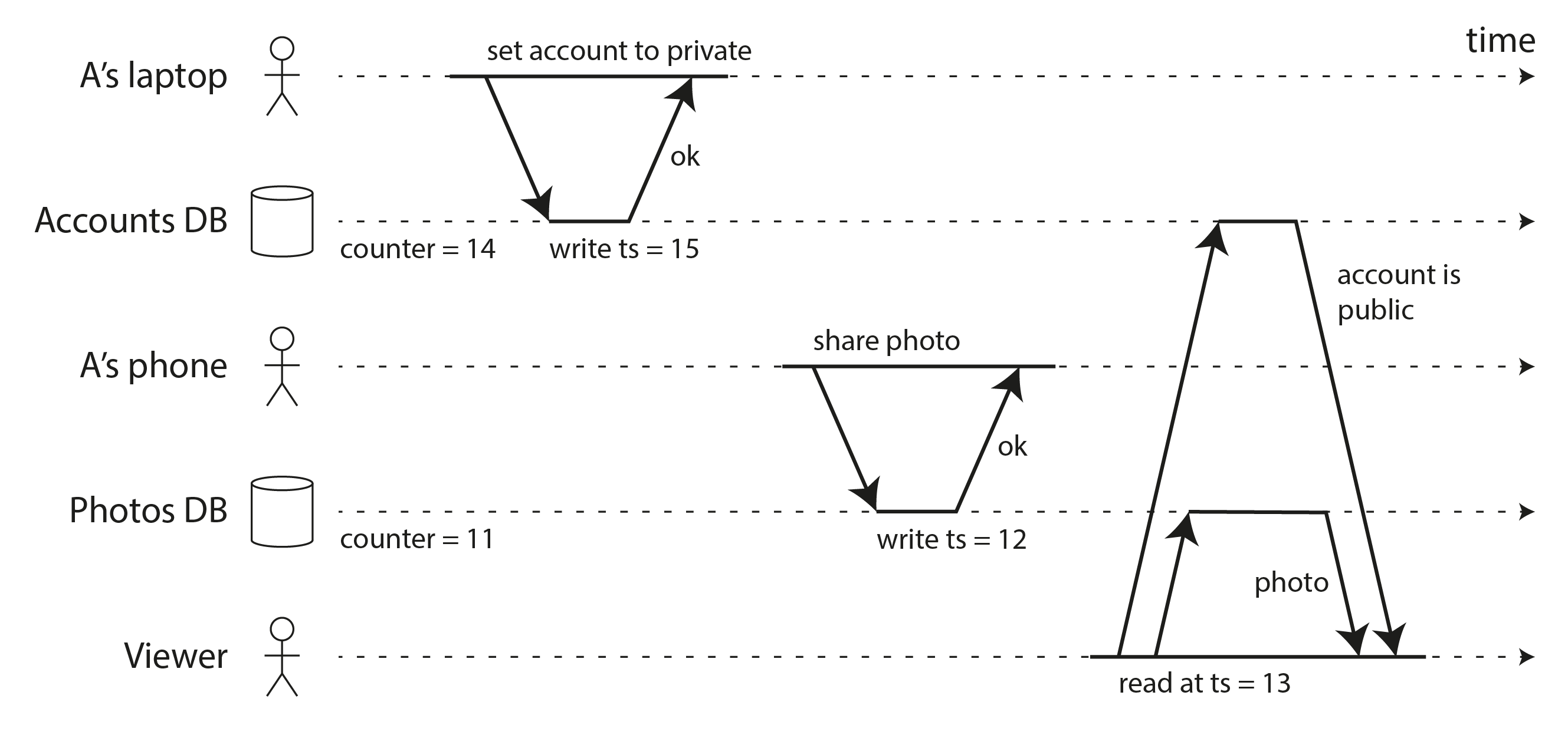
Figure 10-10 User A first sets their account to private, then shares a photo. With a non-linearizable ID generator, an unauthorized viewer may see the photo.

The account permission and the photo are stored in two separate databases (or separate shards of the same database), and let’s assume they use a Lamport clock or hybrid logical clock to assign a timestamp to every write. Since the photos database didn’t read from the accounts database, it’s possible that the local counter in the photos database is slightly behind, and therefore the photo upload is assigned a lower timestamp than the update of the account settings.

Next, let’s say that a viewer (who is not friends with A) is looking at A’s profile, and their read uses an MVCC implementation of snapshot isolation. It could happen that the viewer’s read has a timestamp that is greater than that of the photo upload, but less than that of the account settings update. As a result, the system will determine that the account is still public at the time of the read, and therefore show the viewer the embarrassing photo that they were not supposed to see.

You can imagine several possible ways of fixing this problem. Maybe the photos database should have read the user’s account status before performing the write, but it’s easy to forget such a check. If A’s actions had been performed on the same device, maybe the app on their device could have tracked the latest timestamp of that user’s writes—but if the user uses a laptop and a phone, as in the example, that’s not so easy.

The simplest solution in this case would be to use a linearizable ID generator, which would ensure that the photo upload is assigned a greater ID than the account permissions change.

Implementing a linearizable ID generator

The simplest way of ensuring that ID assignment is linearizable is by actually using a single node for this purpose. That node only needs to atomically increment a counter and return its value when requested, persist the counter value (so that it doesn’t generate duplicate IDs if the node crashes and restarts), and replicate it for fault tolerance (using single-leader replication). This approach is used in practice: for example, TiDB/TiKV calls it a timestamp oracle, inspired by Google’s Percolator ⁵⁷.

As an optimization, you can avoid performing a disk write and replication on every single request. Instead, the ID generator can write a record describing a batch of IDs; once that record is persisted and replicated, the node can start handing out those IDs to clients in sequence. Before it runs out of IDs in that batch, it can persist and replicate the record for the next batch. That way, some IDs will be skipped if the node crashes and restarts or if you fail over to a follower, but you won’t issue any duplicate or out-of-order IDs.

You can’t easily shard the ID generator, since if you have multiple shards independently handing out IDs, you can no longer guarantee that their order is linearizable. You also can’t easily distribute the ID generator across multiple regions; thus, in a geographically distributed database, all requests for IDs will have to go to a node in a single region. On the upside, the ID generator’s job is very simple, so a single node can handle a large request throughput.

If you don’t want to use a single-node ID generator, an alternative is possible: you can do what Google’s Spanner does, as discussed in “Synchronized clocks for global snapshots”. It relies on a physical clock that returns not just a single timestamp, but a range of timestamps indicating the uncertainty in the clock reading. It then waits for the duration of that uncertainty interval to elapse before returning.

Assuming that the uncertainty interval is correct (i.e., that the true current physical time always lies within that interval), this process also ensures that if one request completes before another begins, the later request will have a greater timestamp. This approach ensures this linearizable ID assignment without any communication: even requests in different regions will be ordered correctly, without waiting for cross-region requests. The downside is that you need hardware and software support for clocks to be tightly synchronized and compute the necessary uncertainty interval.

Enforcing constraints using logical clocks

In “Constraints and uniqueness guarantees” we saw that a linearizable compare-and-set operation can be used to implement locks, uniqueness constraints, and similar constructs in a distributed system. This raises the question: is a logical clock or a linearizable ID generator also sufficient to implement these things?

The answer is: not quite. When you have several nodes that are all trying to acquire the same lock or register the same username, you could use a logical clock to assign timestamps to those requests, and pick the one with the lowest timestamp as the winner. If the clock is linearizable, you know that any future requests will always generate greater timestamps, and therefore you can be sure that no future request will receive an even lower timestamp than the winner.

Unfortunately, part of the problem is still unsolved: how does a node know whether its own timestamp is the lowest? To be sure, it needs to hear from every other node that might have generated a timestamp ⁵⁴. If one of the other nodes has failed in the meantime, or cannot be reached due to a network problem, this system would grind to a halt, because we can’t be sure whether that node might have the lowest timestamp. This is not the kind of fault-tolerant system that we need.

To implement locks, leases, and similar constructs in a fault-tolerant way, we need something stronger than logical clocks or ID generators: we need consensus.

Consensus

In this chapter we have seen several examples of things that are easy when you have only a single node, but which get a lot harder if you want fault tolerance:

A database can be linearizable if you have only a single leader, and you make all reads and writes on that leader. But how do you fail over if that leader fails, while avoiding split brain? How do you ensure that a node that believes itself to be the leader hasn’t actually been voted out in the meantime?
A linearizable ID generator on a single node is just a counter with an atomic fetch-and-add instruction, but what if it crashes?
An atomic compare-and-set (CAS) operation is useful for many things, such as deciding who gets a lock or lease when several processes are racing to acquire it, or ensuring the uniqueness of a file or user with a given name. On a single node, CAS may be as simple as one CPU instruction, but how do you make it fault-tolerant?

It turns out that all of these are instances of the same fundamental distributed systems problem: consensus. Consensus is one of the most important and fundamental problems in distributed computing; it is also infamously difficult to get right ⁵⁸ ⁵⁹, and many systems have got it wrong in the past. Now that we have discussed replication (Chapter 6), transactions (Chapter 8), system models (Chapter 9), and linearizability (this chapter), we are finally ready to tackle the consensus problem.

The best-known consensus algorithms are Viewstamped Replication ⁶⁰ ⁶¹, Paxos ⁵⁸ ⁶² ⁶³ ⁶⁴, Raft ²³ ⁶⁵ ⁶⁶, and Zab ¹⁸ ²² ⁶⁷. There are quite a few similarities between these algorithms, but they are not the same ⁶⁸ ⁶⁹. These algorithms work in a non-Byzantine system model: that is, network communication may be arbitrarily delayed or dropped, and nodes may crash, restart, and become disconnected, but the algorithms assume that nodes otherwise follow the protocol correctly and do not behave maliciously.

There are also consensus algorithms that can tolerate some Byzantine nodes, i.e., nodes that don’t correctly follow the protocol (for example, by sending contradictory messages to other nodes). A common assumption is that fewer than one-third of the nodes are Byzantine-faulty ²⁶ ⁷⁰. Such Byzantine fault tolerant (BFT) consensus algorithms are used in blockchains ⁷¹. However, as explained in “Byzantine Faults”, BFT algorithms are beyond the scope of this book.

THE IMPOSSIBILITY OF CONSENSUS

You may have heard about the FLP result ⁷²—named after the authors Fischer, Lynch, and Paterson—which proves that there is no algorithm that is always able to reach consensus if there is a risk that a node may crash. In a distributed system, we must assume that nodes may crash, so reliable consensus is impossible. Yet, here we are, discussing algorithms for achieving consensus. What is going on here?

Firstly, FLP doesn’t say that we can never reach consensus—it only says that we can’t guarantee that a consensus algorithm will always terminate. Moreover, the FLP result is proved assuming a deterministic algorithm in the asynchronous system model (see “System Model and Reality”), which means the algorithm cannot use any clocks or timeouts. If it can use timeouts to suspect that another node may have crashed (even if the suspicion is sometimes wrong), then consensus becomes solvable ⁷³. Even just allowing the algorithm to use random numbers is sufficient to get around the impossibility result ⁷⁴.

Thus, although the FLP result about the impossibility of consensus is of great theoretical importance, distributed systems can usually achieve consensus in practice.

The Many Faces of Consensus

Consensus can be expressed in several different ways:

Single-value consensus is very similar to an atomic compare-and-set operation, and it can be used to implement locks, leases, and uniqueness constraints.
Constructing an append-only log also requires consensus; it is usually formalized as total order broadcast. With a log you can build state machine replication, leader-based replication, event sourcing, and other useful things.
Atomic commitment of a multi-database or multi-shard transaction requires that all participants agree on whether to commit or abort the transaction.

We will explore all of these shortly. In fact, these problems are all equivalent to each other: if you have an algorithm that solves one of these problems, you can convert it into a solution for any of the others. This is quite a profound and perhaps surprising insight! And that’s why we can lump all of these things together under “consensus”, even though they look quite different on the surface.

Single-value consensus

The standard formulation of consensus involves getting multiple nodes to agree on a single value. For example:

When a database with single-leader replication first starts up, or when the existing leader fails, several nodes may concurrently try to become the leader. Similarly, multiple nodes may race to acquire a lock or lease. Consensus allows them to decide which one wins.
If several people concurrently try to book the last seat on an airplane, or the same seat in a theater, or try to register an account with the same username, then a consensus algorithm could determine which one should succeed.

More generally, one or more nodes may propose values, and the consensus algorithm decides on one of those values. In the examples above, each node could propose its own ID, and the algorithm decides which node ID should become the new leader, the holder of the lease, or the buyer of the airplane/theater seat. In this formalism, a consensus algorithm must satisfy the following properties ²⁶:

Uniform agreement: No two nodes decide differently.
Integrity: Once a node has decided one value, it cannot change its mind by deciding another value.
Validity: If a node decides value v, then v was proposed by some node.
Termination: Every node that does not crash eventually decides some value.

If you want to decide multiple values, you can run a separate instance of the consensus algorithm for each. For example, you could have a separate consensus run for each bookable seat in the theater, so that you get one decision (one buyer) for each seat.

The uniform agreement and integrity properties define the core idea of consensus: everyone decides on the same outcome, and once you have decided, you cannot change your mind. The validity property rules out trivial solutions: for example, you could have an algorithm that always decides null, no matter what was proposed; this algorithm would satisfy the agreement and integrity properties, but not the validity property.

If you don’t care about fault tolerance, then satisfying the first three properties is easy: you can just hardcode one node to be the “dictator,” and let that node make all of the decisions. However, if that one node fails, then the system can no longer make any decisions—just like single-leader replication without failover. All the difficulty arises from the need for fault tolerance.

The termination property formalizes the idea of fault tolerance. It essentially says that a consensus algorithm cannot simply sit around and do nothing forever—in other words, it must make progress. Even if some nodes fail, the other nodes must still reach a decision. (Termination is a liveness property, whereas the other three are safety properties—see “Safety and liveness”.)

If a crashed node may recover, you could just wait for it to come back. However, consensus must ensure that it makes a decision even if a crashed node suddenly disappears and never comes back. (Instead of a software crash, imagine that there is an earthquake, and the datacenter containing your node is destroyed by a landslide. You must assume that your node is buried under 30 feet of mud and is never going to come back online.)

Of course, if all nodes crash and none of them are running, then it is not possible for any algorithm to decide anything. There is a limit to the number of failures that an algorithm can tolerate: in fact, it can be proved that any consensus algorithm requires at least a majority of nodes to be functioning correctly in order to assure termination ⁷³. That majority can safely form a quorum (see “Quorums for reading and writing”).

Thus, the termination property is subject to the assumption that fewer than half of the nodes are crashed or unreachable. However, most consensus algorithms ensure that the safety properties—agreement, integrity, and validity—are always met, even if a majority of nodes fail or there is a severe network problem ⁷⁵. Thus, a large-scale outage can stop the system from being able to process requests, but it cannot corrupt the consensus system by causing it to make inconsistent decisions.

Compare-and-set as consensus

A compare-and-set (CAS) operation checks whether the current value of some object equals some expected value; if yes, it atomically updates the object to some new value; if no, it leaves the object unchanged and returns an error.

If you have a fault-tolerant, linearizable CAS operation, it is easy to solve the consensus problem: initially set the object to a null value; each node that wants to propose a value invokes CAS with the expected value being null, and the new value being the value it wants to propose (assuming it is non-null). The decided value is then whatever value the object is set to.

Likewise, if you have a solution for consensus, you can implement CAS: whenever one or more nodes want to perform CAS with the same expected value, you use the consensus protocol to propose the new values in the CAS invocation, and then set the object to whatever value was decided by the consensus. Any CAS invocations whose new value was not decided return an error. CAS invocations with different expected values use separate runs of the consensus protocol.

This shows that CAS and consensus are equivalent to each other ²⁸ ⁷³. Again, both are straightforward on a single node, but challenging to make fault-tolerant. As an example of CAS in a distributed setting, we saw conditional write operations for object stores in “Databases backed by object storage”, which allow a write to happen only if an object with the same name has not been created or modified by another client since the current client last read it.

However, a linearizable read-write register is not sufficient to solve consensus. The FLP result tells us that consensus cannot be solved by a deterministic algorithm in the asynchronous crash-stop model ⁷², but we saw in “Linearizability and quorums” that a linearizable register can be implemented using quorum reads/writes in this model ²⁴ ²⁵ ²⁶. From this it follows that a linearizable register cannot solve consensus.

Shared logs as consensus

We have seen several examples of logs, such as replication logs, transaction logs, and write-ahead logs. A log stores a sequence of log entries, and anyone who reads it sees the same entries in the same order. Sometimes a log has a single writer that is allowed to append new entries, but a shared log is one where multiple nodes can request entries to be appended. An example is single-leader replication: any client can ask the leader to make a write, which the leader appends to the replication log, and then all followers apply the writes in the same order as the leader.

More formally, a shared log supports two operations: you can request for a value to be added to the log, and you can read the entries in the log. It must satisfy the following properties:

Eventual append: If a node requests for some value to be added the log, and the node does not crash, then that node must eventually read that value in a log entry.
Reliable delivery: No log entries are lost: if one node reads some log entry, then eventually every node that does not crash must also read that log entry.
Append-only: Once a node has read some log entry, it is immutable, and new log entries can only be added after it, but not before. A node may re-read the log, in which case it sees the same log entries in the same order as it read them initially (even if the node crashes and restarts).
Agreement: If two nodes both read some log entry e, then prior to e they must have read exactly the same sequence of log entries in the same order.
Validity: If a node reads a log entry containing some value, then some node previously requested for that value to be added to the log.

Note

A shared log is formally known as a total order broadcast, atomic broadcast, or total order multicast protocol ²⁶ ⁷⁶ ⁷⁷ It’s the same thing described in different words: requesting a value to be added to the log is then called “broadcasting” it, and reading a log entry is called “delivering” it.

If you have an implementation of a shared log, it is easy to solve the consensus problem: every node that wants to propose a value requests for it to be added to the log, and whichever value is read back in the first log entry is the value that is decided. Since all nodes read log entries in the same order, they are guaranteed to agree on which value is delivered first ²⁸.

Conversely, if you have a solution for consensus, you can implement a shared log. The details are a bit more complicated, but the basic idea is this ⁷³:

You have a slot in the log for every future log entry, and you run a separate instance of the consensus algorithm for every such slot to decide what value should go in that entry.
When a node wants to add a value to the log, it proposes that value for one of the slots that has not yet been decided.
When the consensus algorithm decides for one of the slots, and all the previous slots have already been decided, then the decided value is appended as a new log entry, and any consecutive slots that have been decided also have their decided value appended to the log.
If a proposed value was not chosen for some slot, the node that wanted to add it retries by proposing it for a later slot.

This shows that consensus is equivalent to total order broadcast and shared logs. Single-leader replication without failover does not meet the liveness requirements, since it stops delivering messages if the leader crashes. As usual, the challenge is in performing failover safely and automatically.

Fetch-and-add as consensus

The linearizable ID generator we saw in “Linearizable ID Generators” comes close to solving consensus, but it falls slightly short. We can implement such an ID generator using a fetch-and-add operation, which atomically increments a counter and returns the old counter value.

If you have a CAS operation, it’s easy to implement fetch-and-add: first read the counter value, then perform a CAS where the expected value is the value you read, and the new value is that value plus one. If the CAS fails, you retry the whole process until the CAS succeeds. This is less efficient than a native fetch-and-add operation when there is contention, but it is functionally equivalent. Since you can implement CAS using consensus, you can also implement fetch-and-add using consensus.

Conversely, if you have a fault-tolerant fetch-and-add operation, can you solve the consensus problem? Let’s say you initialize the counter to zero, and every node that wants to propose a value invokes the fetch-and-add operation to increment the counter. Since the fetch-and-add operation is atomic, one of the nodes will read the initial value of zero, and the others will all read a value that has been incremented at least once.

Now let’s say that the node that reads zero is the winner, and its value is decided. That works for the node that read zero, but the other nodes have a problem: they know that they are not the winner, but they don’t know which of the other nodes has won. The winner could send a message to the other nodes to let them know it has won, but what if the winner crashes before it has a chance to send this message? In that case the other nodes are left hanging, unable to decide any value, and thus the consensus does not terminate. And the other nodes can’t fall back to another node, because the node that read zero may yet come back and rightly decide the value it proposed.

An exception is if we know for sure that no more than two nodes will propose a value. In that case, the nodes can send each other the values they want to propose, and then each perform the fetch-and-add operation. The node that reads zero decides its own value, and the node that reads one decides the other node’s value. This solves the consensus problem among two nodes, which is why we can say that fetch-and-add has a consensus number of two ²⁸. In contrast, CAS and shared logs solve consensus for any number of nodes that may propose values, so they have a consensus number of ∞ (infinity).

Atomic commitment as consensus

In “Distributed Transactions” we saw the atomic commitment problem, which is to ensure that the databases or shards involved in a distributed transaction all either commit or abort a transaction. We also saw the two-phase commit algorithm, which relies on a coordinator that is a single point of failure.

What is the relationship between consensus and atomic commitment? At first glance, they seem very similar—both require nodes to come to some form of agreement. However, there is one important difference: with consensus it’s okay to decide any value that proposed, whereas with atomic commitment the algorithm must abort if any of the participants voted to abort. More precisely, atomic commitment requires the following properties ⁷⁸:

Uniform agreement: No two nodes decide on different outcomes.
Integrity: Once a node has decided one outcome, it cannot change its mind by deciding another outcome.
Validity: If a node decides to commit, then all nodes must have previously voted to commit. If any node voted to abort, the nodes must abort.
Non-triviality: If all nodes vote to commit, and no communication timeouts occur, then all nodes must decide to commit.
Termination: Every node that does not crash eventually decides to either commit or abort.

The validity property ensures that a transaction can only commit if all nodes agree; and the non-triviality property ensures the algorithm can’t simply always abort (but it allows an abort if any of the communication among the nodes times out). The other three properties are basically the same as for consensus.

If you have a solution for consensus, there are multiple ways you could solve atomic commitment ⁷⁸ ⁷⁹. One works like this: when you want to commit the transaction, every node sends its vote to commit or abort to every other node. Nodes that receive a vote to commit from itself and every other node propose “commit” using the consensus algorithm; nodes that receive a vote to abort, or which experience a timeout, propose “abort” using the consensus algorithm. When a node finds out what the consensus algorithm decided, it commits or aborts accordingly.

In this algorithm, “commit” will only be proposed if all nodes voted to commit. If any node voted to abort, all proposals in the consensus algorithm will be “abort”. It could happen that some nodes propose “abort” while others propose “commit” if all nodes voted to commit but some communication timed out; in this case it doesn’t matter whether the nodes commit or abort, as long as they all do the same.

If you have a fault-tolerant atomic commitment protocol, you can also solve consensus. Every node that wants to propose a value starts a transaction on a quorum of nodes, and at each node it performs a single-node CAS to set a register to the proposed value if its value has not already been set by another transaction. If the CAS succeeds, the node votes to commit, otherwise it votes to abort. If the atomic commit protocol decides to commit a transaction, its value is decided for consensus; if atomic commit aborts, the proposing node retries with a new transaction.

This shows that atomic commit and consensus are also equivalent to each other.

Consensus in Practice

We have seen that single-value consensus, CAS, shared logs, and atomic commitment are all equivalent to each other: you can convert a solution to one of them into a solution to any of the others. That is a valuable theoretical insight, but it doesn’t answer the question: which of these many formulations of consensus is the most useful in practice?

The answer is that most consensus systems provide shared logs, also known as total order broadcast. Raft, Viewstamped Replication, and Zab provide shared logs right out of the box. Paxos provides single-value consensus, but in practice most systems using Paxos actually use the extension called Multi-Paxos, which also provides a shared log.

Using shared logs

A shared log is a good fit for database replication: if every log entry represents a write to the database, and every replica processes the same writes in the same order using deterministic logic, then the replicas will all end up in a consistent state. This idea is known as state machine replication ⁸⁰, and it is the principle behind event sourcing, which we saw in “Event Sourcing and CQRS”. Shared logs are also useful for stream processing, as we shall see in Chapter 12.

Similarly, a shared log can be used to implement serializable transactions: as discussed in “Actual Serial Execution”, if every log entry represents a deterministic transaction to be executed as a stored procedure, and if every node executes those transactions in the same order, then the transactions will be serializable ⁸¹ ⁸².

Note

Sharded databases with a strong consistency model often maintain a separate log per shard, which improves scalability, but limits the consistency guarantees (e.g., consistent snapshots, foreign key references) they can offer across shards. Serializable transactions across shards are possible, but require additional coordination ⁸³.

A shared log is also powerful because it can easily be adapted to other forms of consensus:

We saw previously how to use it to implement single-value consensus and CAS: simply decide the value that appears first in the log.
If you want many instances of single-value consensus (e.g. one per seat in a theater that several people are trying to book), include the seat number in the log entries, and decide the first log entry that contains a given seat number.
If you want an atomic fetch-and-add, put the number to add to the counter in a log entry, and the current counter value is the sum of all of the log entries so far. A simple counter on log entries can be used to generate fencing tokens (see “Fencing off zombies and delayed requests”); for example, in ZooKeeper, this sequence number is called zxid ¹⁸.

From single-leader replication to consensus

We saw previously that single-value consensus is easy if you have a single “dictator” node that makes the decision, and likewise a shared log is easy if a single leader is the only node that is allowed to append entries to it. The question is how to provide fault tolerance if that node fails.

Traditionally, databases with single-leader replication didn’t solve this problem: they left leader failover as an action that a human administrator had to perform manually. Unfortunately, this means a significant amount of downtime, since there is a limit to how fast humans can react, and it doesn’t satisfy the termination property of consensus. For consensus, we require that the algorithm can automatically choose a new leader. (Not all consensus algorithms have a leader, but the commonly used algorithms do ⁸⁴.)

However, there is a problem. We previously discussed the problem of split brain, and said that all nodes need to agree who the leader is—otherwise two different nodes could each believe themselves to be the leader, and consequently make inconsistent decisions. Thus, it seems like we need consensus in order to elect a leader, and we need a leader in order to solve consensus. How do we break out of this conundrum?

In fact, consensus algorithms don’t require that there is only one leader at any one time. Instead, they make a weaker guarantee: they define an epoch number (called the ballot number in Paxos, view number in Viewstamped Replication, and term number in Raft) and guarantee that within each epoch, the leader is unique.

When a node believes that the current leader is dead because it hasn’t heard from the leader for some timeout, it may start a vote to elect a new leader. This election is given a new epoch number that is greater than any previous epoch. If there is a conflict between two different leaders in two different epochs (perhaps because the previous leader actually wasn’t dead after all), then the leader with the higher epoch number prevails.

Before a leader is allowed to append the next entry to the shared log, it must first check that there isn’t some other leader with a higher epoch number which might append a different entry. It can do this by collecting votes from a quorum of nodes—typically, but not always, a majority of nodes ⁸⁵. A node votes yes only if it is not aware of any other leader with a higher epoch.

Thus, we have two rounds of voting: once to choose a leader, and a second time to vote on a leader’s proposal for the next entry to append to the log. The quorums for those two votes must overlap: if a vote on a proposal succeeds, at least one of the nodes that voted for it must have also participated in the most recent successful leader election ⁸⁵. Thus, if the vote on a proposal passes without revealing any higher-numbered epoch, the current leader can conclude that no leader with a higher epoch number has been elected, and therefore it can safely append the proposed entry to the log ²⁶ ⁸⁶.

These two rounds of voting look superficially similar to two-phase commit, but they are very different protocols. In consensus algorithms, any node can start an election and it requires only a quorum of nodes to respond; in 2PC, only the coordinator can request votes, and it requires a “yes” vote from every participant before it can commit.

Subtleties of consensus

This basic structure is common to all of Raft, Multi-Paxos, Zab, and Viewstamped Replication: a vote by a quorum of nodes elects a leader, and then another quorum vote is required for every entry that the leader wants to append to the log ⁶⁸ ⁶⁹. Every new log entry is synchronously replicated to a quorum of nodes before it is confirmed to the client that requested the write. This ensures that the log entry won’t be lost if the current leader fails.

However, the devil is in the details, and that’s also where these algorithms take different approaches. For example, when the old leader fails and a new one is elected, the algorithm needs to ensure that the new leader honors any log entries that had already been appended by the old leader before it failed. Raft does this by only allowing a node to become the new leader if its log is at least as up-to-date as a majority of its followers ⁶⁹. In contrast, Paxos allows any node to become the new leader, but requires it to bring its log up-to-date with other nodes before it can start appending new entries of its own.

CONSISTENCY VS. AVAILABILITY IN LEADER ELECTION

If you want the consensus algorithm to strictly guarantee the properties laid out in “Shared logs as consensus”, it’s essential that the new leader is up-to-date with any confirmed log entries before it can process any writes or linearizable reads. If a node with stale data were to become the new leader, it may write a new value to log entries that were already written by the old leader, violating the shared log’s append-only property.

In some cases, you might choose to weaken the consensus properties in order to recover more quickly from a leader failure. For example, Kafka offers the option of enabling unclean leader election, which allows any replica to become leader, even if it is not up-to-date. Also, in databases with asynchronous replication, you cannot guarantee that any follower is up-to-date when the leader fails.

If you drop the requirement for the new leader to be up-to-date, you may improve performance and availability, but you are on thin ice, since the theory of consensus no longer applies. While things will work fine as long as there are no faults, the problems discussed in Chapter 9 can easily cause a lot of data loss or corruption.

Another subtlety is in how the algorithms deal with log entries that had been proposed by the old leader before it failed, but for which the vote on appending to the log had not yet completed. You can find discussions of these details in the references for this chapter ²³ ⁶⁹ ⁸⁶.

For databases that use a consensus algorithm for replication, not only do writes need to be turned into log entries and replicated to a quorum. If you want to guarantee linearizable reads, they also have to go through a quorum vote similarly to a write, to confirm that the node that believes to be the leader really still is up-to-date. Linearizable reads in etcd work like this, for example.

In their standard form, most consensus algorithms assume a fixed set of nodes—that is, nodes may go down and come back up again, but the set of nodes that is allowed to vote is fixed when the cluster is created. In practice, it’s often necessary to add new nodes or remove old nodes in a system configuration. Consensus algorithms have been extended with reconfiguration features that make this possible. This is especially useful when adding new regions to a system, or when migrating from one location to another (by first adding the new nodes, and then removing the old nodes).

Pros and cons of consensus

Although they are complex and subtle, consensus algorithms are a huge breakthrough for distributed systems. Consensus is essentially “single-leader replication done right”, with automatic failover on leader failure, ensuring that no committed data is lost and no split-brain is possible, even in the face of all the problems we discussed in Chapter 9.

Since single-leader replication with automatic failover is essentially one of the definitions of consensus, any system that provides automatic failover but does not use a proven consensus algorithm is likely to be unsafe ⁸⁷. Using a proven consensus algorithm is not a guarantee of correctness of the whole system—there are still plenty of other places where bugs can lurk—but it’s a good start.

Nevertheless, consensus is not used everywhere, because the benefits come at a cost. Consensus systems always require a strict majority to operate—three nodes to tolerate one failure, or five nodes to tolerate two failures. Every operation needs to communicate with a quorum, so you can’t increase throughput by adding more nodes (in fact, every node you add makes the algorithm slower). If a network partition cuts off some nodes from the rest, only the majority portion of the network can make progress, and the rest are blocked.

Consensus systems generally rely on timeouts to detect failed nodes. In environments with highly variable network delays, especially systems distributed across multiple geographic regions, it can be difficult to tune these timeouts: if they are too large it takes a long time to recover from a failure; if they are too small there can be lots of unnecessary leader elections, resulting in terrible performance as the system can end up spending more time choosing leaders than doing useful work.

Sometimes, consensus algorithms are particularly sensitive to network problems. For example, Raft has been shown to have unpleasant edge cases ⁸⁸ ⁸⁹: if the entire network is working correctly except for one particular network link that is consistently unreliable, Raft can get into situations where leadership continually bounces between two nodes, or the current leader is continually forced to resign, so the system effectively never makes progress. Designing algorithms that are more robust to unreliable networks is still an open research problem.

For systems that want to be highly available, but don’t want to accept the cost of consensus, the only real alternative is to use a weaker consistency model instead, such as those offered by leaderless or multi-leader replication as discussed in Chapter 6. These approaches generally don’t offer linearizability, but for applications that don’t need it that is fine.

Coordination Services

Consensus algorithms are useful in any distributed database that wants to offer linearizable operations, and many modern distributed databases use consensus algorithms for replication. But one family of systems is a particularly prominent user of consensus: coordination services such as ZooKeeper, etcd, or Consul. Although these systems look superficially like any other key-value store, they are not designed for general-purpose data storage like most databases.

Instead, they are designed to coordinate between nodes of another distributed system. For example, Kubernetes relies on etcd, while Spark and Flink in high availability mode rely on ZooKeeper running in the background. Coordination services are designed to hold small amounts of data that can fit entirely in memory (although they still write to disk for durability), which is replicated across multiple nodes using a fault-tolerant consensus algorithm.

Coordination services are modeled after Google’s Chubby lock service ¹⁷ ⁵⁸. They combine a consensus algorithm with several other features that turn out to be particularly useful when building distributed systems:

Locks and leases: We saw previously how consensus systems can implement an atomic, fault-tolerant compare-and-set (CAS) operation. Coordination services rely on this approach to implement locks and leases: if several nodes concurrently try to acquire the same lease, only one of them will succeed.
Support for fencing: As discussed in “Distributed Locks and Leases”, when a resource is protected by a lease, you need fencing to prevent clients from interfering with each other in the case of a process pause or large network delay. Consensus systems can generate fencing tokens by giving each log entry a monotonically increasing ID (zxid and cversion in ZooKeeper, revision number in etcd).
Failure detection: Clients maintain a long-lived session on the coordination service, and periodically exchange heartbeats to check if the other node is still alive. Even if the connection is temporarily interrupted, or a server fails, any leases held by the client remain active. However, if there is no heartbeat for longer than the timeout of the lease, the coordination service assumes the client is dead and releases the lease (ZooKeeper calls these ephemeral nodes).
Change notifications: A client can request that the coordination service sends it a notification whenever certain keys change. This allows a client to find out when another client joins the cluster (based on the value it writes to the coordination service), or if another client fails (because its session times out and its ephemeral nodes disappear), for example. These notifications save the client from having to frequently poll the service to find out about changes.

Failure detection and change notifications do not require consensus, but they are useful for distributed coordination alongside the atomic operations and fencing support that do require consensus.

MANAGING CONFIGURATION WITH COORDINATION SERVICES

Applications and infrastructure often have configuration parameters such as timeouts, thread pool sizes, and so on. Coordination services are sometimes used to store such configuration data, represented as key-value pairs. Processes load the latest settings upon startup, and subscribe to receive notifications of any changes. When a configuration changes, the process can begin using the new setting immediately or restart itself to load the latest changes.

Configuration management doesn’t need the consensus aspect of a coordination service, but it’s convenient to use a coordination service and rely on its notification feature if you are already running the coordination service anyway. Alternatively, a process could periodically poll for configuration updates from a file or URL, which avoids the need for a specialized service.

Allocating work to nodes

A coordination service is useful if you have several instances of a process or service, and one of them needs to be chosen as leader or primary. If the leader fails, one of the other nodes should take over. This is necessary for single-leader databases, but it’s also appropriate for job schedulers and similar stateful systems.

Another use case is when you have some sharded resource (database, message streams, file storage, distributed actor system, etc.) and need to decide which shard to assign to which node. As new nodes join the cluster, some of the shards need to be moved from existing nodes to the new nodes in order to rebalance the load. As nodes are removed or fail, other nodes need to take over the failed nodes’ work.

These kinds of tasks can be achieved by judicious use of atomic operations, ephemeral nodes, and notifications in a coordination service. If done correctly, this approach allows the application to automatically recover from faults without human intervention. It’s not easy, despite the appearance of libraries such as Apache Curator that have sprung up to provide higher-level tools on top of the ZooKeeper client API—but it is still much better than attempting to implement the necessary consensus algorithms from scratch, which would be very prone to bugs.

A dedicated coordination service also has the advantage that it can run on a fixed set of nodes (usually three or five), regardless of how many nodes there are in the distributed system that relies on it for coordination. For example, in a storage system with thousands of shards, it would be terribly inefficient to run a consensus algorithm over thousands of nodes; it’s much better to “outsource” the consensus to a small number of nodes running a coordination service.

Normally, the kind of data managed by a coordination service is quite slow-changing: it represents information like “the node running on IP address 10.1.1.23 is the leader for shard 7,” and such assignments usually change on a timescale of minutes or hours. Coordination services are not intended for storing data that may change thousands of times per second. For that, it is better to use a conventional database; alternatively, tools like Apache BookKeeper ⁹⁰ ⁹¹ can be used to replicate fast-changing internal state of a service.

Service discovery

ZooKeeper, etcd, and Consul are also often used for service discovery—that is, to find out which IP address you need to connect to in order to reach a particular service (see “Load balancers, service discovery, and service meshes”). In cloud environments, where it is common for virtual machines to continually come and go, you often don’t know the IP addresses of your services ahead of time. Instead, you can configure your services such that when they start up they register their network endpoints in a service registry, where they can then be found by other services.

Using a coordination service for service discovery can be convenient, as its failure detection and change notification features make it easy for clients to keep track of service instances as they come and go. And if you are already using a coordination service for leases, locking, or leader election, it makes sense to also use it for service discovery, since it already knows which node should receive requests for your service.

However, using consensus for service discovery is often overkill: this use case often doesn’t require linearizability, and it’s more important that service discovery is highly available and fast, since without it everything would grind to a halt. It’s therefore often preferable to cache service discovery information and accept that it might be slightly stale. For example, DNS-based service discovery uses multiple layers of caching to achieve good performance and availability.

To support this use case, ZooKeeper supports observers, which are replicas that receive the log and maintain a copy of the data stored in ZooKeeper, but which do not participate in the consensus algorithm’s voting process. Reads from an observer are not linearizable as they might be stale, but they remain available even if the network is interrupted, and they increase the read throughput that the system can support by caching.

Summary

In this chapter we examined the topic of strong consistency in fault-tolerant systems: what it is, and how to achieve it. We looked in depth at linearizability, a popular formalization of strong consistency: it means that replicated data appears as though there were only a single copy, and all operations act on it atomically. We saw that linearizability is useful when you need some data to be up-to-date when you read it, or if you need to resolve a race condition (e.g. if multiple nodes are concurrently trying to do the same thing, such as creating files with the same name).

Although linearizability is appealing because it is easy to understand—it makes a database behave like a variable in a single-threaded program—it has the downside of being slow, especially in environments with large network delays. Many replication algorithms don’t guarantee linearizability, even though it superficially might seem like they might provide strong consistency.

Next, we applied the concept of linearizability in the context of ID generators. A single-node auto-incrementing counter is linearizable, but not fault-tolerant. Many distributed ID generation schemes don’t guarantee that the IDs are ordered consistently with the order in which the events actually happened. Logical clocks such as Lamport clocks and hybrid logical clocks provide ordering that is consistent with causality, but no linearizability.

This led us to the concept of consensus. We saw that achieving consensus means deciding something in such a way that all nodes agree on what was decided, and such that they can’t change their mind. A wide range of problems are actually reducible to consensus and are equivalent to each other (i.e., if you have a solution for one of them, you can transform it into a solution for all of the others). Such equivalent problems include:

Linearizable compare-and-set operation: The register needs to atomically decide whether to set its value, based on whether its current value equals the parameter given in the operation.
Locks and leases: When several clients are concurrently trying to grab a lock or lease, the lock decides which one successfully acquired it.
Uniqueness constraints: When several transactions concurrently try to create conflicting records with the same key, the constraint must decide which one to allow and which should fail with a constraint violation.
Shared logs: When several nodes concurrently want to append entries to a log, the log decides in which order they are appended. Total order broadcast is also equivalent.
Atomic transaction commit: The database nodes involved in a distributed transaction must all decide the same way whether to commit or abort the transaction.
Linearizable fetch-and-add operation: This operation can be used to implement an ID generator. Several nodes can concurrently invoke the operation, and it decides the order in which they increment the counter. This case actually solves consensus only between two nodes, while the others work for any number of nodes.

All of these are straightforward if you only have a single node, or if you are willing to assign the decision-making capability to a single node. This is what happens in a single-leader database: all the power to make decisions is vested in the leader, which is why such databases are able to provide linearizable operations, uniqueness constraints, a replication log, and more.

However, if that single leader fails, or if a network interruption makes the leader unreachable, such a system becomes unable to make any progress until a human performs a manual failover. Widely-used consensus algorithms like Raft and Paxos are essentially single-leader replication with built-in automatic leader election and failover if the current leader fails.

Consensus algorithms are carefully designed to ensure that no committed writes are lost during a failover, and that the system cannot get into a split brain state in which multiple nodes are accepting writes. This requires that every write, and every linearizable read, is confirmed by a quorum (typically a majority) of nodes. This can be expensive, especially across geographic regions, but it is unavoidable if you want the strong consistency and fault tolerance that consensus provides.

Coordination services like ZooKeeper and etcd are also built on top of consensus algorithms. They provide locks, leases, failure detection, and change notification features that are useful for managing the state of distributed applications. If you find yourself wanting to do one of those things that is reducible to consensus, and you want it to be fault-tolerant, it is advisable to use a coordination service. It won’t guarantee that you will get it right, but it will probably help.

Consensus algorithms are complicated and subtle, but they are supported by a rich body of theory that has been developed since the 1980s. This theory makes it possible to build systems that can tolerate all the faults that we discussed in Chapter 9, and still ensure that your data is not corrupted. This is an amazing achievement, and the references at the end of this chapter feature some of the highlights of this work.

Nevertheless, consensus is not always the right tool: in some systems, the strong consistency properties it provides are not needed, and it is better to have weaker consistency with higher availability and better performance. In these cases, it is common to use leaderless or multi-leader replication, which we previously discussed in Chapter 6. The logical clocks that we discussed in this chapter are helpful in that context.

References

Maurice P. Herlihy and Jeannette M. Wing. Linearizability: A Correctness Condition for Concurrent Objects. ACM Transactions on Programming Languages and Systems (TOPLAS), volume 12, issue 3, pages 463–492, July 1990. doi:10.1145/78969.78972 ↩︎ ↩︎
Leslie Lamport. On interprocess communication. Distributed Computing, volume 1, issue 2, pages 77–101, June 1986. doi:10.1007/BF01786228 ↩︎
David K. Gifford. Information Storage in a Decentralized Computer System. Xerox Palo Alto Research Centers, CSL-81-8, June 1981. Archived at perma.cc/2XXP-3JPB ↩︎
Martin Kleppmann. Please Stop Calling Databases CP or AP. martin.kleppmann.com, May 2015. Archived at perma.cc/MJ5G-75GL ↩︎ ↩︎ ↩︎
Kyle Kingsbury. Call Me Maybe: MongoDB Stale Reads. aphyr.com, April 2015. Archived at perma.cc/DXB4-J4JC ↩︎
Kyle Kingsbury. Computational Techniques in Knossos. aphyr.com, May 2014. Archived at perma.cc/2X5M-EHTU ↩︎
Kyle Kingsbury and Peter Alvaro. Elle: Inferring Isolation Anomalies from Experimental Observations. Proceedings of the VLDB Endowment, volume 14, issue 3, pages 268–280, November 2020. doi:10.14778/3430915.3430918 ↩︎
Paolo Viotti and Marko Vukolić. Consistency in Non-Transactional Distributed Storage Systems. ACM Computing Surveys (CSUR), volume 49, issue 1, article no. 19, June 2016. doi:10.1145/2926965 ↩︎ ↩︎
Peter Bailis. Linearizability Versus Serializability. bailis.org, September 2014. Archived at perma.cc/386B-KAC3 ↩︎
Daniel Abadi. Correctness Anomalies Under Serializable Isolation. dbmsmusings.blogspot.com, June 2019. Archived at perma.cc/JGS7-BZFY ↩︎
Peter Bailis, Aaron Davidson, Alan Fekete, Ali Ghodsi, Joseph M. Hellerstein, and Ion Stoica. Highly Available Transactions: Virtues and Limitations. Proceedings of the VLDB Endowment, volume 7, issue 3, pages 181–192, November 2013. doi:10.14778/2732232.2732237, extended version published as arXiv:1302.0309 ↩︎
Philip A. Bernstein, Vassos Hadzilacos, and Nathan Goodman. Concurrency Control and Recovery in Database Systems. Addison-Wesley, 1987. ISBN: 978-0-201-10715-9, available online at microsoft.com. ↩︎
Andrei Matei. CockroachDB’s consistency model. cockroachlabs.com, February 2021. Archived at perma.cc/MR38-883B ↩︎
Murat Demirbas. Strict-serializability, but at what cost, for what purpose? muratbuffalo.blogspot.com, August 2022. Archived at perma.cc/T8AY-N3U9 ↩︎
Ben Darnell. How to talk about consistency and isolation in distributed DBs. cockroachlabs.com, February 2022. Archived at perma.cc/53SV-JBGK ↩︎
Daniel Abadi. An explanation of the difference between Isolation levels vs. Consistency levels. dbmsmusings.blogspot.com, August 2019. Archived at perma.cc/QSF2-CD4P ↩︎
Mike Burrows. The Chubby Lock Service for Loosely-Coupled Distributed Systems. At 7th USENIX Symposium on Operating System Design and Implementation (OSDI), November 2006. ↩︎ ↩︎
Flavio P. Junqueira and Benjamin Reed. ZooKeeper: Distributed Process Coordination. O’Reilly Media, 2013. ISBN: 978-1-449-36130-3 ↩︎ ↩︎ ↩︎ ↩︎
Murali Vallath. Oracle 10g RAC Grid, Services & Clustering. Elsevier Digital Press, 2006. ISBN: 978-1-555-58321-7 ↩︎ ↩︎
Peter Bailis, Alan Fekete, Michael J. Franklin, Ali Ghodsi, Joseph M. Hellerstein, and Ion Stoica. Coordination Avoidance in Database Systems. Proceedings of the VLDB Endowment, volume 8, issue 3, pages 185–196, November 2014. doi:10.14778/2735508.2735509 ↩︎
Kyle Kingsbury. Call Me Maybe: etcd and Consul. aphyr.com, June 2014. Archived at perma.cc/XL7U-378K ↩︎
Flavio P. Junqueira, Benjamin C. Reed, and Marco Serafini. Zab: High-Performance Broadcast for Primary-Backup Systems. At 41st IEEE International Conference on Dependable Systems and Networks (DSN), June 2011. doi:10.1109/DSN.2011.5958223 ↩︎ ↩︎
Diego Ongaro and John K. Ousterhout. In Search of an Understandable Consensus Algorithm. At USENIX Annual Technical Conference (ATC), June 2014. ↩︎ ↩︎ ↩︎
Hagit Attiya, Amotz Bar-Noy, and Danny Dolev. Sharing Memory Robustly in Message-Passing Systems. Journal of the ACM, volume 42, issue 1, pages 124–142, January 1995. doi:10.1145/200836.200869 ↩︎ ↩︎
Nancy Lynch and Alex Shvartsman. Robust Emulation of Shared Memory Using Dynamic Quorum-Acknowledged Broadcasts. At 27th Annual International Symposium on Fault-Tolerant Computing (FTCS), June 1997. doi:10.1109/FTCS.1997.614100 ↩︎ ↩︎
Christian Cachin, Rachid Guerraoui, and Luís Rodrigues. Introduction to Reliable and Secure Distributed Programming, 2nd edition. Springer, 2011. ISBN: 978-3-642-15259-7, doi:10.1007/978-3-642-15260-3 ↩︎ ↩︎ ↩︎ ↩︎ ↩︎ ↩︎
Niklas Ekström, Mikhail Panchenko, and Jonathan Ellis. Possible Issue with Read Repair? Email thread on cassandra-dev mailing list, October 2012. ↩︎
Maurice P. Herlihy. Wait-Free Synchronization. ACM Transactions on Programming Languages and Systems (TOPLAS), volume 13, issue 1, pages 124–149, January 1991. doi:10.1145/114005.102808 ↩︎ ↩︎ ↩︎ ↩︎
Armando Fox and Eric A. Brewer. Harvest, Yield, and Scalable Tolerant Systems. At 7th Workshop on Hot Topics in Operating Systems (HotOS), March 1999. doi:10.1109/HOTOS.1999.798396 ↩︎
Seth Gilbert and Nancy Lynch. Brewer’s Conjecture and the Feasibility of Consistent, Available, Partition-Tolerant Web Services. ACM SIGACT News, volume 33, issue 2, pages 51–59, June 2002. doi:10.1145/564585.564601 ↩︎ ↩︎ ↩︎
Seth Gilbert and Nancy Lynch. Perspectives on the CAP Theorem. IEEE Computer Magazine, volume 45, issue 2, pages 30–36, February 2012. doi:10.1109/MC.2011.389 ↩︎
Eric A. Brewer. CAP Twelve Years Later: How the ‘Rules’ Have Changed. IEEE Computer Magazine, volume 45, issue 2, pages 23–29, February 2012. doi:10.1109/MC.2012.37 ↩︎ ↩︎
Susan B. Davidson, Hector Garcia-Molina, and Dale Skeen. Consistency in Partitioned Networks. ACM Computing Surveys, volume 17, issue 3, pages 341–370, September 1985. doi:10.1145/5505.5508 ↩︎
Paul R. Johnson and Robert H. Thomas. RFC 677: The Maintenance of Duplicate Databases. Network Working Group, January 1975. ↩︎
Michael J. Fischer and Alan Michael. Sacrificing Serializability to Attain High Availability of Data in an Unreliable Network. At 1st ACM Symposium on Principles of Database Systems (PODS), March 1982. doi:10.1145/588111.588124 ↩︎
Eric A. Brewer. NoSQL: Past, Present, Future. At QCon San Francisco, November 2012. ↩︎
Adrian Cockcroft. Migrating to Microservices. At QCon London, March 2014. ↩︎
Martin Kleppmann. A Critique of the CAP Theorem. arXiv:1509.05393, September 2015. ↩︎ ↩︎
Daniel Abadi. Problems with CAP, and Yahoo’s little known NoSQL system. dbmsmusings.blogspot.com, April 2010. Archived at perma.cc/4NTZ-CLM9 ↩︎ ↩︎ ↩︎
Daniel Abadi. Hazelcast and the Mythical PA/EC System. dbmsmusings.blogspot.com, October 2017. Archived at perma.cc/J5XM-U5C2 ↩︎ ↩︎
Eric Brewer. Spanner, TrueTime & The CAP Theorem. research.google.com, February 2017. Archived at perma.cc/59UW-RH7N ↩︎
Daniel J. Abadi. Consistency Tradeoffs in Modern Distributed Database System Design. IEEE Computer Magazine, volume 45, issue 2, pages 37–42, February 2012. doi:10.1109/MC.2012.33 ↩︎ ↩︎
Nancy A. Lynch. A Hundred Impossibility Proofs for Distributed Computing. At 8th ACM Symposium on Principles of Distributed Computing (PODC), August 1989. doi:10.1145/72981.72982 ↩︎
Prince Mahajan, Lorenzo Alvisi, and Mike Dahlin. Consistency, Availability, and Convergence. University of Texas at Austin, Department of Computer Science, Tech Report UTCS TR-11-22, May 2011. Archived at perma.cc/SAV8-9JAJ ↩︎
Hagit Attiya, Faith Ellen, and Adam Morrison. Limitations of Highly-Available Eventually-Consistent Data Stores. At ACM Symposium on Principles of Distributed Computing (PODC), July 2015. doi:10.1145/2767386.2767419 ↩︎
Peter Sewell, Susmit Sarkar, Scott Owens, Francesco Zappa Nardelli, and Magnus O. Myreen. x86-TSO: A Rigorous and Usable Programmer’s Model for x86 Multiprocessors. Communications of the ACM, volume 53, issue 7, pages 89–97, July 2010. doi:10.1145/1785414.1785443 ↩︎
Martin Thompson. Memory Barriers/Fences. mechanical-sympathy.blogspot.co.uk, July 2011. Archived at perma.cc/7NXM-GC5U ↩︎
Ulrich Drepper. What Every Programmer Should Know About Memory. akkadia.org, November 2007. Archived at perma.cc/NU6Q-DRXZ ↩︎
Hagit Attiya and Jennifer L. Welch. Sequential Consistency Versus Linearizability. ACM Transactions on Computer Systems (TOCS), volume 12, issue 2, pages 91–122, May 1994. doi:10.1145/176575.176576 ↩︎
Kyzer R. Davis, Brad G. Peabody, and Paul J. Leach. Universally Unique IDentifiers (UUIDs). RFC 9562, IETF, May 2024. ↩︎ ↩︎
Ryan King. Announcing Snowflake. blog.x.com, June 2010. Archived at archive.org ↩︎
Alizain Feerasta. Universally Unique Lexicographically Sortable Identifier. github.com, 2016. Archived at perma.cc/NV2Y-ZP8U ↩︎
Rob Conery. A Better ID Generator for PostgreSQL. bigmachine.io, May 2014. Archived at perma.cc/K7QV-3KFC ↩︎
Leslie Lamport. Time, Clocks, and the Ordering of Events in a Distributed System. Communications of the ACM, volume 21, issue 7, pages 558–565, July 1978. doi:10.1145/359545.359563 ↩︎ ↩︎
Sandeep S. Kulkarni, Murat Demirbas, Deepak Madeppa, Bharadwaj Avva, and Marcelo Leone. Logical Physical Clocks. 18th International Conference on Principles of Distributed Systems (OPODIS), December 2014. doi:10.1007/978-3-319-14472-6_2 ↩︎
Manuel Bravo, Nuno Diegues, Jingna Zeng, Paolo Romano, and Luís Rodrigues. On the use of Clocks to Enforce Consistency in the Cloud. IEEE Data Engineering Bulletin, volume 38, issue 1, pages 18–31, March 2015. Archived at perma.cc/68ZU-45SH ↩︎
Daniel Peng and Frank Dabek. Large-Scale Incremental Processing Using Distributed Transactions and Notifications. At 9th USENIX Conference on Operating Systems Design and Implementation (OSDI), October 2010. ↩︎
Tushar Deepak Chandra, Robert Griesemer, and Joshua Redstone. Paxos Made Live – An Engineering Perspective. At 26th ACM Symposium on Principles of Distributed Computing (PODC), June 2007. doi:10.1145/1281100.1281103 ↩︎ ↩︎ ↩︎
Will Portnoy. Lessons Learned from Implementing Paxos. blog.willportnoy.com, June 2012. Archived at perma.cc/QHD9-FDD2 ↩︎
Brian M. Oki and Barbara H. Liskov. Viewstamped Replication: A New Primary Copy Method to Support Highly-Available Distributed Systems. At 7th ACM Symposium on Principles of Distributed Computing (PODC), August 1988. doi:10.1145/62546.62549 ↩︎
Barbara H. Liskov and James Cowling. Viewstamped Replication Revisited. Massachusetts Institute of Technology, Tech Report MIT-CSAIL-TR-2012-021, July 2012. Archived at perma.cc/56SJ-WENQ ↩︎
Leslie Lamport. The Part-Time Parliament. ACM Transactions on Computer Systems, volume 16, issue 2, pages 133–169, May 1998. doi:10.1145/279227.279229 ↩︎
Leslie Lamport. Paxos Made Simple. ACM SIGACT News, volume 32, issue 4, pages 51–58, December 2001. Archived at perma.cc/82HP-MNKE ↩︎
Robbert van Renesse and Deniz Altinbuken. Paxos Made Moderately Complex. ACM Computing Surveys (CSUR), volume 47, issue 3, article no. 42, February 2015. doi:10.1145/2673577 ↩︎
Diego Ongaro. Consensus: Bridging Theory and Practice. PhD Thesis, Stanford University, August 2014. Archived at perma.cc/5VTZ-2ADH ↩︎
Heidi Howard, Malte Schwarzkopf, Anil Madhavapeddy, and Jon Crowcroft. Raft Refloated: Do We Have Consensus? ACM SIGOPS Operating Systems Review, volume 49, issue 1, pages 12–21, January 2015. doi:10.1145/2723872.2723876 ↩︎
André Medeiros. ZooKeeper’s Atomic Broadcast Protocol: Theory and Practice. Aalto University School of Science, March 2012. Archived at perma.cc/FVL4-JMVA ↩︎
Robbert van Renesse, Nicolas Schiper, and Fred B. Schneider. Vive La Différence: Paxos vs. Viewstamped Replication vs. Zab. IEEE Transactions on Dependable and Secure Computing, volume 12, issue 4, pages 472–484, September 2014. doi:10.1109/TDSC.2014.2355848 ↩︎ ↩︎
Heidi Howard and Richard Mortier. Paxos vs Raft: Have we reached consensus on distributed consensus?. At 7th Workshop on Principles and Practice of Consistency for Distributed Data (PaPoC), April 2020. doi:10.1145/3380787.3393681 ↩︎ ↩︎ ↩︎ ↩︎
Miguel Castro and Barbara H. Liskov. Practical Byzantine Fault Tolerance and Proactive Recovery. ACM Transactions on Computer Systems, volume 20, issue 4, pages 396–461, November 2002. doi:10.1145/571637.571640 ↩︎
Shehar Bano, Alberto Sonnino, Mustafa Al-Bassam, Sarah Azouvi, Patrick McCorry, Sarah Meiklejohn, and George Danezis. SoK: Consensus in the Age of Blockchains. At 1st ACM Conference on Advances in Financial Technologies (AFT), October 2019. doi:10.1145/3318041.3355458 ↩︎
Michael J. Fischer, Nancy Lynch, and Michael S. Paterson. Impossibility of Distributed Consensus with One Faulty Process. Journal of the ACM, volume 32, issue 2, pages 374–382, April 1985. doi:10.1145/3149.214121 ↩︎ ↩︎
Tushar Deepak Chandra and Sam Toueg. Unreliable Failure Detectors for Reliable Distributed Systems. Journal of the ACM, volume 43, issue 2, pages 225–267, March 1996. doi:10.1145/226643.226647 ↩︎ ↩︎ ↩︎ ↩︎
Michael Ben-Or. Another Advantage of Free Choice: Completely Asynchronous Agreement Protocols. At 2nd ACM Symposium on Principles of Distributed Computing (PODC), August 1983. doi:10.1145/800221.806707 ↩︎
Cynthia Dwork, Nancy Lynch, and Larry Stockmeyer. Consensus in the Presence of Partial Synchrony. Journal of the ACM, volume 35, issue 2, pages 288–323, April 1988. doi:10.1145/42282.42283 ↩︎
Xavier Défago, André Schiper, and Péter Urbán. Total Order Broadcast and Multicast Algorithms: Taxonomy and Survey. ACM Computing Surveys, volume 36, issue 4, pages 372–421, December 2004. doi:10.1145/1041680.1041682 ↩︎
Hagit Attiya and Jennifer Welch. Distributed Computing: Fundamentals, Simulations and Advanced Topics, 2nd edition. John Wiley & Sons, 2004. ISBN: 978-0-471-45324-6, doi:10.1002/0471478210 ↩︎
Rachid Guerraoui. Revisiting the Relationship Between Non-Blocking Atomic Commitment and Consensus. At 9th International Workshop on Distributed Algorithms (WDAG), September 1995. doi:10.1007/BFb0022140 ↩︎ ↩︎
Jim N. Gray and Leslie Lamport. Consensus on Transaction Commit. ACM Transactions on Database Systems (TODS), volume 31, issue 1, pages 133–160, March 2006. doi:10.1145/1132863.1132867 ↩︎
Fred B. Schneider. Implementing Fault-Tolerant Services Using the State Machine Approach: A Tutorial. ACM Computing Surveys, volume 22, issue 4, pages 299–319, December 1990. doi:10.1145/98163.98167 ↩︎
Alexander Thomson, Thaddeus Diamond, Shu-Chun Weng, Kun Ren, Philip Shao, and Daniel J. Abadi. Calvin: Fast Distributed Transactions for Partitioned Database Systems. At ACM International Conference on Management of Data (SIGMOD), May 2012. doi:10.1145/2213836.2213838 ↩︎
Mahesh Balakrishnan, Dahlia Malkhi, Ted Wobber, Ming Wu, Vijayan Prabhakaran, Michael Wei, John D. Davis, Sriram Rao, Tao Zou, and Aviad Zuck. Tango: Distributed Data Structures over a Shared Log. At 24th ACM Symposium on Operating Systems Principles (SOSP), November 2013. doi:10.1145/2517349.2522732 ↩︎
Mahesh Balakrishnan, Dahlia Malkhi, Vijayan Prabhakaran, Ted Wobber, Michael Wei, and John D. Davis. CORFU: A Shared Log Design for Flash Clusters. At 9th USENIX Symposium on Networked Systems Design and Implementation (NSDI), April 2012. ↩︎
Vasilis Gavrielatos, Antonios Katsarakis, and Vijay Nagarajan. Odyssey: the impact of modern hardware on strongly-consistent replication protocols. At 16th European Conference on Computer Systems (EuroSys), April 2021. doi:10.1145/3447786.3456240 ↩︎
Heidi Howard, Dahlia Malkhi, and Alexander Spiegelman. Flexible Paxos: Quorum Intersection Revisited. At 20th International Conference on Principles of Distributed Systems (OPODIS), December 2016. doi:10.4230/LIPIcs.OPODIS.2016.25 ↩︎ ↩︎
Martin Kleppmann. Distributed Systems lecture notes. University of Cambridge, October 2024. Archived at perma.cc/SS3Q-FNS5 ↩︎ ↩︎
Kyle Kingsbury. Call Me Maybe: Elasticsearch 1.5.0. aphyr.com, April 2015. Archived at perma.cc/37MZ-JT7H ↩︎
Heidi Howard and Jon Crowcroft. Coracle: Evaluating Consensus at the Internet Edge. At Annual Conference of the ACM Special Interest Group on Data Communication (SIGCOMM), August 2015. doi:10.1145/2829988.2790010 ↩︎
Tom Lianza and Chris Snook. A Byzantine failure in the real world. blog.cloudflare.com, November 2020. Archived at perma.cc/83EZ-ALCY ↩︎
Ivan Kelly. BookKeeper Tutorial. github.com, October 2014. Archived at perma.cc/37Y6-VZWU ↩︎
Jack Vanlightly. Apache BookKeeper Insights Part 1 — External Consensus and Dynamic Membership. medium.com, November 2021. Archived at perma.cc/3MDB-8GFB ↩︎

PART III: Derived Data

In Parts I and II of this book, we assembled from the ground up all the major considerations that go into a distributed database, from the layout of data on disk all the way to the limits of distributed consistency in the presence of faults. However, this discussion assumed that there was only one database in the application.

In reality, data systems are often more complex. In a large application you often need to be able to access and process data in many different ways, and there is no one database that can satisfy all those different needs simultaneously. Applications thus commonly use a combination of several different datastores, indexes, caches, analytics systems, etc. and implement mechanisms for moving data from one store to another.

In this final part of the book, we will examine the issues around integrating multiple different data systems, potentially with different data models and optimized for different access patterns, into one coherent application architecture. This aspect of system-building is often overlooked by vendors who claim that their product can satisfy all your needs. In reality, integrating disparate systems is one of the most important things that needs to be done in a nontrivial application.

Systems of Record and Derived Data

On a high level, systems that store and process data can be grouped into two broad categories:

Systems of record

A system of record, also known as source of truth, holds the authoritative version of your data. When new data comes in, e.g., as user input, it is first written here. Each fact is represented exactly once (the representation is typically normalized). If there is any discrepancy between another system and the system of record, then the value in the system of record is (by definition) the correct one.

Derived data systems

Data in a derived system is the result of taking some existing data from another system and transforming or processing it in some way. If you lose derived data, you can recreate it from the original source. A classic example is a cache: data can be served from the cache if present, but if the cache doesn’t contain what you need, you can fall back to the underlying database. Denormalized values, indexes, and materialized views also fall into this category. In recommendation systems, predictive summary data is often derived from usage logs.

Technically speaking, derived data is redundant, in the sense that it duplicates existing information. However, it is often essential for getting good performance on read queries. It is commonly denormalized. You can derive several different datasets from a single source, enabling you to look at the data from different “points of view.”

Not all systems make a clear distinction between systems of record and derived data in their architecture, but it’s a very helpful distinction to make, because it clarifies the dataflow through your system: it makes explicit which parts of the system have which inputs and which outputs, and how they depend on each other.

Most databases, storage engines, and query languages are not inherently either a system of record or a derived system. A database is just a tool: how you use it is up to you. The distinction between system of record and derived data system depends not on the tool, but on how you use it in your application.

By being clear about which data is derived from which other data, you can bring clarity to an otherwise confusing system architecture. This point will be a running theme throughout this part of the book.

Overview of Chapters

We will start in Chapter 11 by examining batch-oriented dataflow systems such as MapReduce, and see how they give us good tools and principles for building large- scale data systems. In Chapter 12 we will take those ideas and apply them to data streams, which allow us to do the same kinds of things with lower delays. In Chapter 13 we explore ideas about how we might use these tools to build reliable, scalable, and maintainable applications in the future. Chapter 14 concludes the book with ethics, privacy, and the social impact of data systems.

Chapters

11. Batch Processing

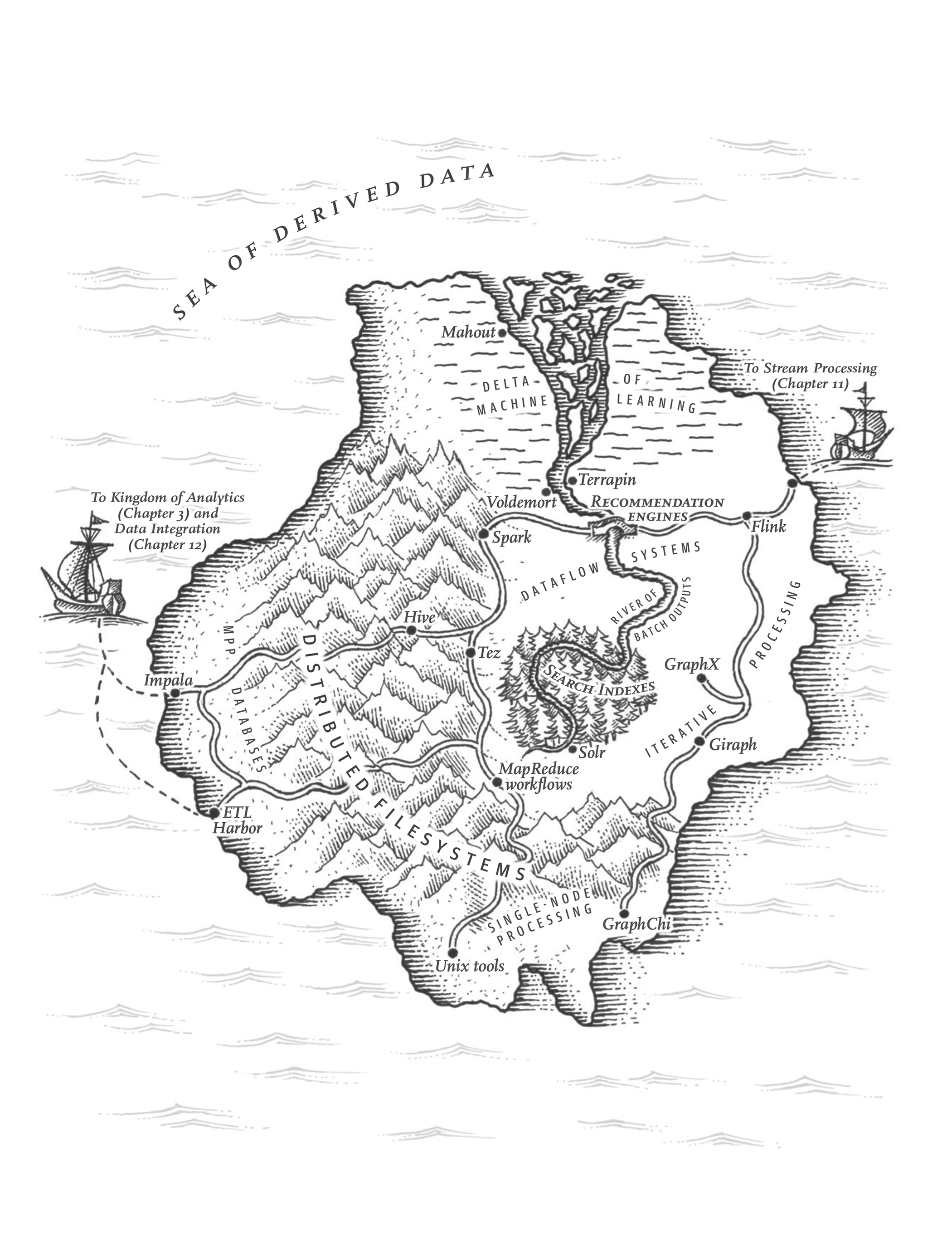
A system cannot be successful if it is too strongly influenced by a single person. Once the initial design is complete and fairly robust, the real test begins as people with many different viewpoints undertake their own experiments.

Donald Knuth

A NOTE FOR EARLY RELEASE READERS

This will be the 11th chapter of the final book. The GitHub repo for this book is https://github.com/ept/ddia2-feedback.

If you’d like to be actively involved in reviewing and commenting on this draft, please reach out on GitHub.

Much of this book so far has talked about requests and queries, and the corresponding responses or results. This style of data processing is assumed in many modern data systems: you ask for something, or you send an instruction, and the system tries to give you an answer as quickly as possible.

A web browser requesting a page, a service calling a remote API, databases, caches, search indexes, and many other systems work this way. We call these online systems. Response time is usually their primary measure of performance, and they often require fault tolerance to ensure high availability.

However, sometimes you need to run a bigger computation or process larger amounts of data than you can do in an interactive request. Maybe you need to train an AI model, or transform lots of data from one form into another, or compute analytics over a very large dataset. We call these tasks batch processing jobs, or sometimes offline systems.

A batch processing job takes some input data (which is read-only), and produces some output data (which is generated from scratch every time the job runs). It typically does not mutate data in the way a read/write transaction would. The output is therefore derived from the input (as discussed in “Systems of Record and Derived Data”): if you don’t like the output, you can just delete it, adjust the job logic, and run it again. By treating inputs as immutable and avoiding side effects (such as writing to external databases), batch jobs not only achieve good performance but also have other benefits:

If you introduce a bug into the code and the output is wrong or corrupted, you can simply roll back to a previous version of the code and rerun the job, and the output will be correct again. Or, even simpler, you can keep the old output in a different directory and simply switch back to it. Most object stores and open table formats (see “Cloud Data Warehouses”) support this feature, which is known as time travel. Most databases with read-write transactions do not have this property: if you deploy buggy code that writes bad data to the database, then rolling back the code will do nothing to fix the data in the database. The idea of being able to recover from buggy code has been called human fault tolerance ¹.
As a consequence of this ease of rolling back, feature development can proceed more quickly than in an environment where mistakes could mean irreversible damage. This principle of minimizing irreversibility is beneficial for Agile software development ².
The same set of files can be used as input for various different jobs, including monitoring jobs that calculate metrics and evaluate whether a job’s output has the expected characteristics (for example, by comparing it to the output from the previous run and measuring discrepancies).
Batch processing frameworks make efficient use of computing resources. Even though it’s possible to batch process data using online data systems such as OLTP databases and applications servers, doing so can be much more expensive in terms of the resources required.

Batch data processing also presents challenges. With most frameworks, output can only be processed by other jobs after the whole job finishes. Batch processing can also be inefficient: any change to input data—even a single byte—means the batch job must reprocess the entire input dataset. Despite these limitations, batch processing has proven useful in a wide range of use cases, which we’ll revisit in “Batch Use Cases”.

A batch job may take a long time to run: minutes, hours, or even days. Jobs may be scheduled to run periodically (for example, once per day). The primary measure of performance is usually throughput: how much data the job can process per unit time. Some batch systems handle faults by simply aborting and restarting the whole job, while others have fault tolerance so that a job can complete successfully despite some of its nodes crashing.

Note

An alternative to batch processing is stream processing, in which the job doesn’t finish running when it has processed the input, but instead continues watching the input and processes changes in the input shortly after they happen. We will turn to stream processing in Chapter 12.

The boundary between online and batch processing systems is not always clear: a long-running database query looks quite like a batch process. But batch processing also has some particular characteristics that make it a useful building block for building reliable, scalable, and maintainable applications. For example, it often plays a role in data integration, i.e., composing multiple data systems to achieve things that one system alone cannot do. ETL, as discussed in “Data Warehousing”, is an example of this.

Modern batch processing has been heavily influenced by MapReduce, a batch processing algorithm that was published by Google in 2004 ³, and subsequently implemented in various open source data systems, including Hadoop, CouchDB, and MongoDB. MapReduce is a fairly low-level programming model, and less sophisticated than the parallel query execution engines found, for example, in data warehouses ⁴, ⁵. When it was new, MapReduce was a step forward in terms of the scale of processing that could be achieved on commodity hardware, but now it is largely obsolete, and no longer used at Google ⁶, ⁷.

Batch processing today is more often done using frameworks such as Spark or Flink, or data warehouse query engines. Like MapReduce, they rely heavily on sharding (see Chapter 7) and parallel execution, but they have far more sophisticated caching and execution strategies. As these systems have matured, operational concerns have been largely solved, so focus has shifted toward usability. New processing models such as dataflow APIs, query languages, and DataFrame APIs are now widely supported. Job and workflow orchestration has also matured. Hadoop-centric workflow schedulers such as Oozie and Azkaban have been replaced with more generalized solutions such as Airflow, Dagster, and Prefect, which support a wide array of batch processing frameworks and cloud data warehouses.

Cloud computing has grown ubiquitous. Batch storage layers are shifting from distributed filesystems (DFSs) like HDFS, GlusterFS, and CephFS to object storage systems such as S3. Scalable cloud data warehouses like BigQuery and Snowflake are blurring the line between data warehouses and batch processing.

To build an intuition of what batch processing is about, we will start this chapter with an example that uses standard Unix tools on a single machine. We will then investigate how we can extend data processing to multiple machines in a distributed system. We will see that, much like an operating system, distributed batch processing frameworks have a scheduler and a filesystem. We will then explore various processing models that we use to write batch jobs. Finally, we discuss common batch processing use cases.

Batch Processing with Unix Tools

Say you have a web server that appends a line to a log file every time it serves a request. For example, using the nginx default access log format, one line of the log might look like this:

216.58.210.78 - - [27/Jun/2025:17:55:11 +0000] "GET /css/typography.css HTTP/1.1"
200 3377 "https://martin.kleppmann.com/" "Mozilla/5.0 (Macintosh; Intel Mac OS X
10_15_7) AppleWebKit/537.36 (KHTML, like Gecko) Chrome/137.0.0.0 Safari/537.36"

(That is actually one line; it’s only broken onto multiple lines here for readability.) There’s a lot of information in that line. In order to interpret it, you need to look at the definition of the log format, which is as follows:

$remote_addr - $remote_user [$time_local] "$request"
$status $body_bytes_sent "$http_referer" "$http_user_agent"

So, this one line of the log indicates that on June 27, 2025, at 17:55:11 UTC, the server received a request for the file /css/typography.css from the client IP address 216.58.210.78. The user was not authenticated, so $remote_user is set to a hyphen (-). The response status was 200 (i.e., the request was successful), and the response was 3,377 bytes in size. The web browser was Chrome 137, and it loaded the file because it was referenced in the page at the URL https://martin.kleppmann.com/.

Though log parsing might seem contrived, it’s actually a critical part of many modern technology companies, and is used for everything from ad pipelines to payment processing. Indeed, it was a driving force behind the rapid adoption of MapReduce and the “big data” movement.

Simple Log Analysis

Various tools can take these log files and produce pretty reports about your website traffic, but for the sake of exercise, let’s build our own, using basic Unix tools. For example, say you want to find the five most popular pages on your website. You can do this in a Unix shell as follows:

cat /var/log/nginx/access.log | #1
  awk '{print $7}' | #2
  sort             | #3
  uniq -c          | #4
  sort -r -n       | #5
  head -n 5          #6

Read the log file. (Strictly speaking, cat is unnecessary here, as the input file could be given directly as an argument to awk. However, the linear pipeline is more apparent when written like this.)
Split each line into fields by whitespace, and output only the seventh such field from each line, which happens to be the requested URL. In our example line, this request URL is /css/typography.css.
Alphabetically sort the list of requested URLs. If some URL has been requested n times, then after sorting, the file contains the same URL repeated n times in a row.
The uniq command filters out repeated lines in its input by checking whether two adjacent lines are the same. The -c option tells it to also output a counter: for every distinct URL, it reports how many times that URL appeared in the input.
The second sort sorts by the number (-n) at the start of each line, which is the number of times the URL was requested. It then returns the results in reverse (-r) order, i.e. with the largest number first.
Finally, head outputs just the first five lines (-n 5) of input, and discards the rest.

The output of that series of commands looks something like this:

4189 /favicon.ico
3631 /2016/02/08/how-to-do-distributed-locking.html
2124 /2020/11/18/distributed-systems-and-elliptic-curves.html
1369 /
 915 /css/typography.css

Although the preceding command line likely looks a bit obscure if you’re unfamiliar with Unix tools, it is incredibly powerful. It will process gigabytes of log files in a matter of seconds, and you can easily modify the analysis to suit your needs. For example, if you want to omit CSS files from the report, change the awk argument to '$7 !~ /\.css$/ {print $7}'. If you want to count top client IP addresses instead of top pages, change the awk argument to '{print $1}'. And so on.

We don’t have space in this book to explore Unix tools in detail, but they are very much worth learning about. Surprisingly many data analyses can be done in a few minutes using some combination of awk, sed, grep, sort, uniq, and xargs, and they perform surprisingly well ⁸.

Chain of Commands Versus Custom Program

Instead of the chain of Unix commands, you could write a simple program to do the same thing. For example, in Python, it might look something like this:

from collections import defaultdict

counts = defaultdict(int) #1

with open('/var/log/nginx/access.log', 'r') as file:
    for line in file:
        url = line.split()[6] #2
        counts[url] += 1 #3

top5 = sorted(((count, url) for url, count in counts.items()), reverse=True)[:5] #4

for count, url in top5:  #5
    print(f"{count} {url}")

counts is a hash table that keeps a counter for the number of times we’ve seen each URL. A counter is zero by default.
From each line of the log, we take the URL to be the seventh whitespace-separated field (the array index is 6 because Python’s arrays are zero-indexed).
Increment the counter for the URL in the current line of the log.
Sort the hash table contents by counter value (descending), and take the top five entries.
Print out those top five entries.

This program is not as concise as the chain of Unix pipes, but it’s fairly readable, and which of the two you prefer is partly a matter of taste. However, besides the superficial syntactic differences between the two, there is a big difference in the execution flow, which becomes apparent if you run this analysis on a large file.

Sorting Versus In-memory Aggregation

The Python script keeps an in-memory hash table of URLs, where each URL is mapped to the number of times it has been seen. The Unix pipeline example does not have such a hash table, but instead relies on sorting a list of URLs in which multiple occurrences of the same URL are simply repeated.

Which approach is better? It depends how many different URLs you have. For most small to mid-sized websites, you can probably fit all distinct URLs, and a counter for each URL, in (say) 1 GB of memory. In this example, the working set of the job (the amount of memory to which the job needs random access) depends only on the number of distinct URLs: if there are a million log entries for a single URL, the space required in the hash table is still just one URL plus the size of the counter. If this working set is small enough, an in-memory hash table works fine—even on a laptop.

On the other hand, if the job’s working set is larger than the available memory, the sorting approach has the advantage that it can make efficient use of disks. It’s the same principle as we discussed in “Log-Structured Storage”: chunks of data can be sorted in memory and written out to disk as segment files, and then multiple sorted segments can be merged into a larger sorted file. Mergesort has sequential access patterns that perform well on disks (see “Sequential Versus Random Writes on SSDs”).

The sort utility in GNU Coreutils (Linux) automatically handles larger-than-memory datasets by spilling to disk, and automatically parallelizes sorting across multiple CPU cores ⁹. This means that the simple chain of Unix commands we saw earlier easily scales to large datasets, without running out of memory. The bottleneck is likely to be the rate at which the input file can be read from disk.

A limitation of Unix tools is that they run only on a single machine. Datasets that are too large to fit in memory or local disk present a problem—and that’s where distributed batch processing frameworks come in.

Batch Processing in Distributed Systems

The machine that runs our Unix tool example has a number of components that work together to process the log data:

Storage devices that are accessed through the operating system’s filesystem interface.
A scheduler that determines when processes get to run, and how to allocate CPU resources to them.
A series of Unix programs whose stdin and stdout are connected together by pipes.

These same components exist in distributed data processing frameworks. In fact, you can think of a distributed processing framework as a distributed operating system; they have filesystems, job schedulers, and programs that send data to each other through the filesystem or other communication channels.

Distributed Filesystems

The filesystem provided by your operating system is composed of several layers:

At the lowest level, block device drivers speak directly to the disk, and allow the layers above to read and write raw blocks.
Above the block layer sits a page cache that keeps recently accessed blocks in memory for faster access.
The block API is wrapped in a filesystem layer that breaks up large files into blocks, and tracks file metadata such as inodes, directories, and files. ext4 and XFS are two common implementations on Linux, for example.
Finally, the operating system exposes different filesystems to applications through a common API called the virtual file system (VFS). The VFS is what allows applications to read and write in a standard way regardless of the underlying filesystem.

Distributed filesystems work in much the same way. Files are broken up into blocks, which are distributed across many machines. DFS blocks are typically much larger than local blocks: HDFS (Hadoop Distributed File System) defaults to 128MB, while JuiceFS and many object stores use 4MB blocks—much larger than ext4’s 4096 bytes. Larger blocks mean less metadata to keep track of, which makes a big difference on petabyte-sized datasets. Larger blocks also lower the overhead of seeking to a block relative to reading it.

Most physical storage devices can’t write partial blocks, so operating systems require writes to use an entire block even if the data doesn’t take up the whole block. Since distributed filesystems have larger blocks and are usually implemented on top of operating system filesystems, they don’t have this requirement. For example, a 900MB file stored with 128MB blocks would have 7 blocks that use 128MB and 1 block that uses 4MB.

DFS blocks are read by making network requests to a machine in the cluster that stores the block. Each machine runs a daemon, exposing an API that allows remote processes to read and write blocks as files on its local filesystem. HDFS refers to these daemons as DataNodes, while GlusterFS calls them glusterfsd processes. We’ll call them data nodes in this book.

Distributed filesystems also implement the distributed equivalent of a page cache. Since DFS blocks are stored as files on data nodes, reads and writes go through each data node’s operating system, which includes an in-memory page cache. This keeps frequently read data blocks in-memory on the data nodes. Some distributed filesystems also implement more caching tiers such as the client-side and local-disk caching found in JuiceFS.

Filesystems such as ext4 and XFS keep track of storage metadata including free space, file block locations, directory structures, permission settings, and more. Distributed filesystems also need a way to track file locations spread across machines, permission settings, and so on. Hadoop has a service called the NameNode, which maintains metadata for the cluster. DeepSeek’s 3FS has a metadata service that persists its data to a key-value store such as FoundationDB.

Above the filesystem sits the VFS. A close analogue in batch processing is a distributed filesystem’s protocol. Distributed filesystems must expose a protocol or interface so that batch processing systems can read and write files. This protocol acts as a pluggable interface: any DFS may be used so long as it implements the protocol. For example, Amazon S3’s API has been widely adopted by other storage systems such as MinIO, Cloudflare’s R2, Tigris, Backblaze’s B2, and many others. Batch processing systems with S3 support can use any of these storage systems.

Some DFSs implement POSIX-compliant filesystems that appear to the operating system’s VFS like any other filesystem. Filesystem in Userspace (FUSE) or the Network File System (NFS) protocol are often used to integrate into the VFS. NFS is perhaps the most well known distributed filesystem protocol. The protocol was originally developed to allow multiple clients to read and write data on a single server. More recently, filesystems such as AWS’s Elastic File System (EFS) and Archil provide NFS-compatible distributed filesystem implementations that are far more scalable. NFS clients still connect to one end point, but underneath, these systems communicate with distributed metadata services and data nodes to read and write data.

DISTRIBUTED FILESYSTEMS AND NETWORK STORAGE

Distributed filesystems are based on the shared-nothing principle (see “Shared-Memory, Shared-Disk, and Shared-Nothing Architecture”), in contrast to the shared-disk approach of Network Attached Storage (NAS) and Storage Area Network (SAN) architectures. Shared-disk storage is implemented by a centralized storage appliance, often using custom hardware and special network infrastructure such as Fibre Channel. On the other hand, the shared-nothing approach requires no special hardware, only computers connected by a conventional datacenter network.

Many distributed filesystems are built on commodity hardware, which is less expensive but has higher failure rates than enterprise-grade hardware. In order to tolerate machine and disk failures, file blocks are replicated on multiple machines. This also allows schedulers to more evenly distribute workloads since it can execute a task on any node that contains a replica of the task’s input data. Replication may mean simply several copies of the same data on multiple machines, as in Chapter 6, or an erasure coding scheme such as Reed–Solomon codes, which allows lost data to be recovered with lower storage overhead than full replication ¹⁰, ¹¹, ¹². The techniques are similar to RAID, which provides redundancy across several disks attached to the same machine; the difference is that in a distributed filesystem, file access and replication are done over a conventional datacenter network without special hardware.

Object Stores

Object storage services such as Amazon S3, Google Cloud Storage, Azure Blob Storage, and OpenStack Swift have become a popular alternative to distributed filesystems for batch processing jobs. In fact, the line between the two is somewhat blurry. As we saw in the previous section and “Databases Backed by Object Storage”, Filesystem in Userspace (FUSE) drivers allow users to treat object stores such as S3 as a filesystem. Some DFS implementations such as JuiceFS and Ceph offer both object storage and filesystem APIs. However, their APIs, performance, and consistency guarantees are very different. Care must be taken when adopting such systems to make sure they behave as expected, even if they seem to implement the requisite APIs.

Each object in an object store has a URL such as s3://my-photo-bucket/2025/04/01/birthday.png. The host portion of the URL (my-photo-bucket) describes the bucket where objects are stored, and the part that follows is the object’s key (/2025/04/01/birthday.png in our example). A bucket has a globally unique name, and each object’s key must be unique within its bucket.

Objects are read using a get call and written using a put call. Unlike files on a filesystem, objects are immutable once written. To update an object, it must be fully rewritten using a put call, similarly to a key-value store. Azure Blob Storage and S3 Express One Zone support appends, but most other stores do not. There are no file handle APIs with functions like fopen and fseek.

Objects may look as if they are organised into directories, which is somewhat confusing, since object stores do not have the concept of directories. The path structure is simply a convention, and the slashes are a part of the object’s key. This convention allows you to perform something similar to a directory listing by requesting a list of objects with a particular prefix. However, listing objects by prefix is different from a filesystem directory listing in two ways:

A prefix list operation behaves like recursive ls -R call on a Unix system: it returns all objects that start with the prefix—objects in subpaths are included.
Empty directories are not possible: if you were to remove all objects underneath s3://my-photo-bucket/2025/04/01, then 01 would no longer appear when we call list on s3://my-photo-bucket/2025/04. It is a common practice to create a zero-byte object as a way to represent an empty directory (e.g. creating an empty s3://my-photo-bucket/2025/04/01 file to keep it present when all child objects are deleted).

DFS implementations often support many common filesystem operations such as hard links, symbolic links, file locking, and atomic renames. Such features are missing from object stores. Linking and locks are typically not supported, while renames are non-atomic; they’re accomplished by copying the object to the new key, and then deleting the old object. If you want to rename a directory, you have to individually rename every object within it, since the directory name is a part of the key.

The key-value stores we discussed in Chapter 4 are optimized for small values (typically kilobytes) and frequent, low-latency reads/writes. In contrast, distributed filesystems and object stores are generally optimized for large objects (megabytes to gigabytes) and less frequent, larger reads. Recently, however, object stores have begun to add support for frequent and smaller reads/writes. For example, S3 Express One Zone now offers single-millisecond latency and a pricing model that is more similar to key-value stores.

Another difference between distributed filesystems and object stores is that DFSes such as HDFS allow computing tasks to be run on the machine that stores a copy of a particular file. This allows the task to read that file without having to send it over the network, which saves bandwidth if the executable code of the task is smaller than the file it needs to read. On the other hand, object stores usually keep storage and computation separate. Doing so might use more bandwidth, but modern datacenter networks are very fast, so this is often acceptable. This architecture also allows machine resources such as CPU and memory to be scaled independently of storage since the two are decoupled.

Distributed Job Orchestration

Our operating system analogy also applies to job orchestration. When you execute a Unix batch job, something needs to actually run the awk, sort, uniq, and head processes. Data needs to be transferred from one process’s output to another process’s input, memory must be allocated for each process, instructions from each process must be scheduled fairly and executed on the CPU, memory and I/O boundaries must be enforced, and so on. On a single machine, an operating system’s kernel is responsible for such work. In a distributed environment, this is the role of a job orchestrator.

Batch processing frameworks send a request to an orchestrator’s scheduler to run a job. Requests to start a job contain metadata such as:

the number of tasks to execute,
the amount of memory, CPU, and disk needed for each task,
a job identifier,
access credentials,
job paramaters such as input and output data,
required hardware details such as GPUs or disk types, and
where the job’s executable code is located.

Orchestrators such as Kubernetes and Hadoop YARN (Yet Another Resource Negotiator) ¹³ combine this information with cluster metadata to execute the job using the following components:

Task executors

An executor daemon such as YARN’s NodeManager or Kubernetes’s kubelet runs on each node in the cluster. Executors are responsible for running job tasks, sending heartbeats to signal their liveness, and tracking task status and resource allocation on the node. When a task-start request is sent to an executor, it retrieves the job’s executable code and runs a command to start the task. The executor then monitors the process until it finishes or fails, at which point it updates the task status metadata accordingly.

Many executors also work with the operating system to provide both security and performance isolation. YARN and Kubernetes both use Linux cgroups, for example. This prevents tasks from accessing data without permission, or from negatively affecting the performance of other tasks on the node by using excessive resources.

Resource Manager

An orchestrator’s resource manager stores metadata about each node, including available hardware (CPUs, GPUs, memory, disks, and so on), task statuses, network location, node status, and other relevant information. Thus, the manager provides a global view of the cluster’s current state. The centralized nature of the resource manager can lead to both scalability and availability bottlenecks. YARN uses ZooKeeper and Kubernetes uses etcd to store cluster state (see “Coordination Services”).

Scheduler

Orchestrators usually have a centralized scheduler subsystem, which receives requests to start, stop, or check on the status of a job. For example, a scheduler might receive a request to start a job with 10 tasks using a specific Docker image on nodes that have a specific type of GPU. The scheduler uses the information from the request and state of the resource manager to determine which tasks to run on which nodes. The task executors are then informed of their assigned work and begin execution.

Though each orchestrator uses different terminology, you will find these components in nearly all orchestration systems.

Note

Scheduling decisions sometimes require application-specific schedulers that can take into account particular requirements, such as auto-scaling read replicas when a certain query threshold is reached. The centralized scheduler and application-specific schedulers work together to determine how to best execute tasks. YARN refers to its sub-schedulers as ApplicationMasters, while Kubernetes calls them operators.

Resource Allocation

Schedulers have a particularly challenging role in job orchestration: they must figure out how to best allocate the cluster’s limited resources amongst jobs with competing needs. Fundamentally, its decisions must balance fairness and efficiency.

Imagine a small cluster with five nodes that has a total of 160 CPU cores available. The cluster’s scheduler receives two job requests, each wanting 100 cores to complete its work. What’s the best way to schedule the workload?

The scheduler could decide to run 80 tasks for each job, starting the remaining 20 tasks for each job as earlier tasks complete.
The scheduler could run all of one job’s tasks, and begin running the second job’s tasks only when 100 cores are available, a strategy known as gang scheduling.
One job request comes before the other. The scheduler has to decide whether to allocate all 100 cores to that job, or hold some back in anticipation for future jobs.

This is a very simple example, but we already see many difficult trade-offs. In the gang-scheduling scenario, for example, if the scheduler reserves CPU cores until all 100 are available at the same time, nodes will sit idle. The cluster’s resource utilization will drop and a deadlock might occur if other jobs also attempt to reserve CPU cores.

On the other hand, if the scheduler simply waits for 100 cores to become available, other jobs might grab the cores in the meantime. The cluster might not have 100 cores available for a very long time, which leads to starvation. The scheduler could decide to preempt some of the first job’s tasks, killing them to make room for the second job. Task preemption decreases cluster efficiency as well, since the killed tasks will need to be restarted later and re-run.

Now imagine a scheduler that must make allocation decisions for hundreds or even millions of such job requests. Finding an optimal solution seems intractable. In fact, the problem is NP-hard, which means that it is prohibitively slow to calculate an optimal solution for all but the smallest examples ¹⁴, ¹⁵.

In practice, schedulers therefore use heuristics to make non-optimal but reasonable decisions. Several algorithms are commonly used, including first-in first-out (FIFO), dominant resource fairness (DRF), priority queues, capacity or quota-based scheduling, and various bin-packing algorithms. The details for such algorithms are beyond the scope of this book, but they’re a fascinating area of research.

Scheduling Workflows

The Unix tools example at the start of this chapter involved a chain of several commands, connected by Unix pipes. The same pattern arises in distributed batch processes: often the output from one job needs to become the input to one or more other jobs, and each job may have several inputs that are produced by other jobs. This is called a workflow or directed acyclic graph (DAG) of jobs.

Note

In “Durable Execution and Workflows” we saw workflow engines that offer durable execution of a sequence of steps, typically performing RPCs. In the context of batch processing, “workflow” has a different meaning: it’s a sequence of batch processes, each taking input data and producing output data, but normally not making RPCs to external services. Durable execution engines typically process less data per-request than their batch processing counterparts, though the line is somewhat fuzzy.

There are several reasons why a workflow of multiple jobs might be needed:

If the output of one job needs to become the input to several other jobs, which are maintained by different teams, it’s best for the first job to first write its output to a location where all the other jobs can read it. Those consuming jobs can then be scheduled to run every time that data has been updated, or on some other schedule.
You might want to transfer data from one processing tool to another. For example, a Spark job might output its data to HDFS, then a Python script might trigger a Trino SQL query (see “Cloud Data Warehouses”) that does further processing on the HDFS files and outputs to S3.
Some data pipelines internally require multiple processing stages. For example, if one stage needs to shard the data by one key, and the next stage needs to shard by a different key, the first stage can output data sharded in the way that is required by the second stage.

In the Unix tools example, the pipe that connects the output of one command to the input of another uses only a small in-memory buffer, and doesn’t write the data into a file. If that buffer fills up, the producing process needs to wait until the consuming process has read some data from the buffer before it can output more—a form of backpressure. Spark, Flink, and other batch execution engines support a similar model where the output of one task is directly passed to another task (over the network if the tasks are running on different machines).

However, in a workflow it is more usual for one job to write its output to a distributed filesystem or object store, and for the next job to read it from there. This decouples the jobs from each other, allowing them to run at different times. If a job has several inputs, a workflow scheduler typically waits until all of the jobs that produce its inputs have completed successfully before running the job that consumes those inputs.

Schedulers found in orchestration frameworks such as YARN’s ResourceManager or Spark’s built-in scheduler do not manage entire workflows; they do scheduling on a per-job basis. To handle these dependencies between job executions, various workflow schedulers have been developed, including Airflow, Dagster, and Prefect. Workflow schedulers have management features that are useful when maintaining a large collection of batch jobs. Workflows consisting of 50 to 100 jobs are common in many data pipelines, and in a large organization, many different teams may be running different jobs or workflows that read each other’s output across many different systems. Tool support is important for managing such complex dataflows.

Handling Faults

Batch jobs often run for long periods of time. Long-running jobs with many parallel tasks are likely to experience at least one task failure along the way. As discussed in “Hardware and Software Faults” and “Unreliable Networks”, there are many reasons why this could happen, including hardware faults (especially on commodity hardware), or network interruptions.

Another reason why a task might not finish running is that the scheduler may intentionally preempt (kill) it. Preemption is particularly useful if you have multiple priority levels: low-priority tasks that are cheaper to run, and high-priority tasks that cost more. Low-priority tasks can run whenever there is spare computing capacity, but they run the risk of being preempted at any moment if a higher-priority task arrives. Such cheaper, low-priority virtual machines are called spot instances on Amazon EC2, spot virtual machines on Azure, and preemptible instances on Google Cloud ¹⁶.

Since batch processing is often used for jobs that are not time-sensitive, it is well suited for using low-priority tasks and spot instances to reduce the cost of running jobs. Essentially, those jobs can use spare computing resources that would otherwise be idle, and thereby increase the utilization of the cluster. However, this also means that those tasks are more likely to be killed by the scheduler: preemptions occur more frequently than hardware faults ¹⁷.

Since batch jobs regenerate their output from scratch every time they are run, task failures are easier to handle than in online systems: the system can delete the partial output from the failed execution and schedule it to run again on another machine. It would be wasteful to rerun the entire job due to a single task failure, though. MapReduce and its successors therefore keep the execution of parallel tasks independent from each other, so that they can retry work at the granularity of an individual task ³.

Fault tolerance is trickier when the output of one task becomes the input to another task as part of a workflow. MapReduce solves this by always writing such intermediate data back to the distributed filesystem, and waiting for the writing task to complete successfully before allowing other tasks to read the data. This works, even in an environment where preemption is common, but it means a lot of writes to the DFS, which can be inefficient.

Spark keeps intermediate data in memory or “spills” to local disk, and only writes the final result to the DFS. It also keeps track of how the intermediate data was computed, allowing Spark to recompute it in case it is lost ¹⁸. Flink uses a different approach based on periodically checkpointing a snapshot of tasks ¹⁹. We will return to this topic in “Dataflow Engines”.

Batch Processing Models

We have seen how batch jobs are scheduled in a distributed environment. Let us now turn our attention to how batch processing frameworks actually process data. The two most common models are MapReduce and dataflow engines. Although dataflow engines have largely replaced MapReduce in practice, it is useful to understand how MapReduce works, since it influenced many modern batch processing frameworks.

MapReduce and dataflow engines have evolved to support multiple programming models including low-level programmatic APIs, relational query languages, and DataFrame APIs. A variety of options enable application engineers, analytics engineers, business analysts, and even non-technical employees to process company data for various use cases, which we’ll discuss in “Batch Use Cases”.

MapReduce

The pattern of data processing in MapReduce is very similar to the web server log analysis example in “Simple Log Analysis”:

Read a set of input files, and break it up into records. In the web server log example, each record is one line in the log (that is, \n is the record separator). In Hadoop’s MapReduce, the input file is stored in a distributed filesystem like HDFS or an object store like S3. Various file formats are used, such as Apache Parquet (a columnar format, see “Column-Oriented Storage”) or Apache Avro (a row-based format, see “Avro”).
Call the mapper function to extract a key and value from each input record. In the Unix tool example, the mapper function is awk '{print $7}': it extracts the URL ($7) as the key, and leaves the value empty.
Sort all of the key-value pairs by key. In the log example, this is done by the first sort command.
Call the reducer function to iterate over the sorted key-value pairs. If there are multiple occurrences of the same key, the sorting has made them adjacent in the list, so it is easy to combine those values without having to keep a lot of state in memory. In the Unix tool example, the reducer is implemented by the command uniq -c, which counts the number of adjacent records with the same key.

Those four steps can be performed by one MapReduce job. Steps 2 (map) and 4 (reduce) are where you write your custom data processing code. Step 1 (breaking files into records) is handled by the input format parser. Step 3, the sort step, is implicit in MapReduce—you don’t have to write it, because the output from the mapper is always sorted before it is given to the reducer. This sorting step is a foundational batch processing algorithm, which we’ll revisit in “Shuffling Data”.

To create a MapReduce job, you need to implement two callback functions, the mapper and reducer, which behave as follows:

Mapper: The mapper is called once for every input record, and its job is to extract the key and value from the input record. For each input, it may generate any number of key-value pairs (including none). It does not keep any state from one input record to the next, so each record is handled independently.
Reducer: The MapReduce framework takes the key-value pairs produced by the mappers, collects all the values belonging to the same key, and calls the reducer with an iterator over that collection of values. The reducer can produce output records (such as the number of occurrences of the same URL).

In the web server log example, we had a second sort command in step 5, which ranked URLs by number of requests. In MapReduce, if you need a second sorting stage, you can implement it by writing a second MapReduce job and using the output of the first job as input to the second job. Viewed like this, the role of the mapper is to prepare the data by putting it into a form that is suitable for sorting, and the role of the reducer is to process the data that has been sorted.

MAPREDUCE AND FUNCTIONAL PROGRAMMING

Though MapReduce is used for batch processing, the programming model comes from functional programming. Lisp introduced map and reduce (or fold) as higher‑order functions on lists, and they have made their way into mainstream languages such as Python, Rust, and Java. Many common data processing operations, including those offered by SQL, can be implemented on top of MapReduce. Both functions, and functional programming in general, have important properties that MapReduce benefits from. Map and reduce are composable, which fits nicely with data processing (as we saw in our Unix example). Map is also embarrassingly parallel (each input is processed independently), which simplifies MapReduce’s parallel execution. For reduce, different keys can be processed in parallel.

Implementing a complex processing job using the raw MapReduce APIs is actually quite hard and laborious—for instance, any join algorithms used by the job would need to be implemented from scratch ²⁰. MapReduce is also quite slow compared to more modern batch processors. One reason is that its file-based I/O prevents job pipelining, i.e., processing output data in a downstream job before the upstream job is complete.

Dataflow Engines

In order to fix some of MapReduce’s problems, several new execution engines for distributed batch computations were developed, the most well known of which are Spark ¹⁸, ²¹ and Flink ¹⁹. There are various differences in the way they are designed, but they have one thing in common: they handle an entire workflow as one job, rather than breaking it up into independent subjobs.

Since they explicitly model the flow of data through several processing stages, these systems are known as dataflow engines. Like MapReduce, they support a low-level API that repeatedly calls a user-defined function to process one record at a time, but they also offer higher-level operators such as join and group by. They parallelize work by sharding inputs, and they copy the output of one task over the network to become the input to another task. Unlike in MapReduce, operators need not take the strict roles of alternating map and reduce, but instead can be assembled in more flexible ways.

These dataflow APIs generally use relational-style building blocks to express a computation: joining datasets on the value of some field; grouping tuples by key; filtering by some condition; and aggregating tuples by counting, summing, or other functions. Internally, these operations are implemented using the shuffle algorithms that we discuss in the next section.

This style of processing engine is based on research systems like Dryad ²² and Nephele ²³, and it offers several advantages compared to the MapReduce model:

Expensive work such as sorting need only be performed in places where it is actually required, rather than always happening by default between every map and reduce stage.
When there are several operators in a row that don’t change the sharding of the dataset (such as map or filter), they can be combined into a single task, reducing data copying overheads.
Because all joins and data dependencies in a workflow are explicitly declared, the scheduler has an overview of what data is required where, so it can make locality optimizations. For example, it can try to place the task that consumes some data on the same machine as the task that produces it, so that the data can be exchanged through a shared memory buffer rather than having to copy it over the network.
It is usually sufficient for intermediate state between operators to be kept in memory or written to local disk, which requires less I/O than writing it to a distributed filesystem or object store (where it must be replicated to several machines and written to disk on each replica). MapReduce already uses this optimization for mapper output, but dataflow engines generalize the idea to all intermediate state.
Operators can start executing as soon as their input is ready; there is no need to wait for the entire preceding stage to finish before the next one starts.
Existing processes can be reused to run new operators, reducing startup overheads compared to MapReduce (which launches a new JVM for each task).

You can use dataflow engines to implement the same computations as MapReduce workflows, and they usually execute significantly faster due to the optimizations described here.

Shuffling Data

We saw that both the Unix tools example at the beginning of the chapter and MapReduce are based on sorting. Batch processors need to be able to sort datasets petabytes in size, which are too large to fit on a single machine. They therefore require a distributed sorting algorithm where both the input and the output is sharded. Such an algorithm is called a shuffle.

SHUFFLE IS NOT RANDOM

The term shuffle is confusing. When you shuffle a deck of cards, you end up with a random order. In contrast, the shuffle we’re talking about here produces a sorted order, with no randomness.

Shuffling is a foundational algorithm for batch processors, where it is used for joins and aggregations. MapReduce, Spark, Flink, Daft, Dataflow, and BigQuery ²⁴ all implement scalable and performant shuffle algorithms in order to handle large datasets. We’ll use the shuffle in Hadoop MapReduce ²⁵ for illustration purposes, but the concepts in this section translate to other systems as well.

Figure 11-1 shows the dataflow in a MapReduce job. We assume that the input to the job is sharded, and the shards are labelled m 1, m 2, and m 3. For example, each shard may be a separate file on HDFS or a separate object in an object store, and all the shards belonging to the same dataset are grouped into the same HDFS directory or have the same key prefix in an object store bucket.

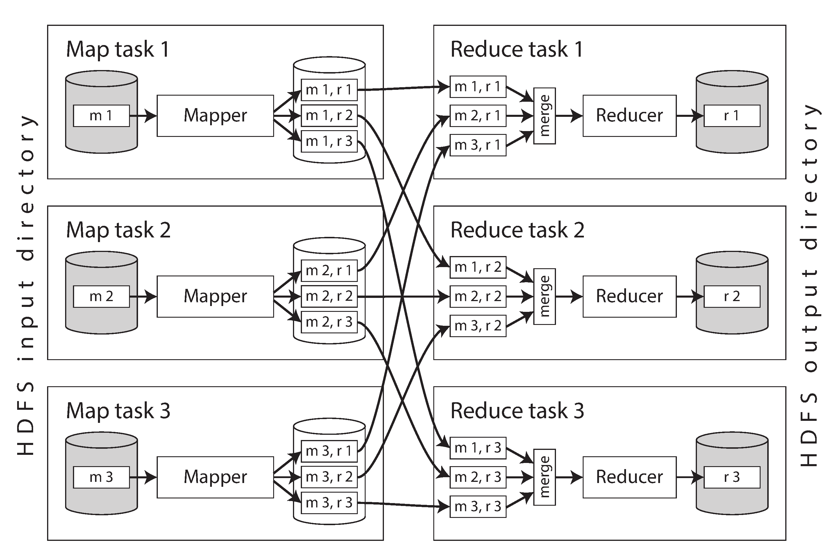
Figure 11-1 A MapReduce job with three mappers and three reducers.

The framework starts a separate map task for each input shard. A task reads its assigned file, passing one record at a time to the mapper callback. The reduce side of the computation is also sharded. While the number of map tasks is determined by the number of input shards, the number of reduce tasks is configured by the job author (it can be different from the number of map tasks).

The output of the mapper consists of key-value pairs, and the framework needs to ensure that if two different mappers output the same key, those key-value pairs end up being processed by the same reducer task. To achieve this, each mapper creates a separate output file on its local disk for every reducer (for example, the file m 1, r 2 in Figure 11-1 is the file created by mapper 1 containing the data destined for reducer 2). When the mapper outputs a key-value pair, a hash of the key typically determines which reducer file it is written to (similarly to “Sharding by Hash of Key”).

While a mapper is writing these files, it also sorts the key-value pairs within each file. This can be done using the techniques we saw in “Log-Structured Storage”: batches of key-value pairs are first collected in a sorted data structure in memory, then written out as sorted segment files, and smaller segment files are progressively merged into larger ones.

After each mapper finishes, reducers connect to it and copy the appropriate file of sorted key-value pairs to their local disk. Once the reduce task has its share of the output from all of the mappers, it merges these files together, preserving the sort order, mergesort-style. Key-value pairs with the same key are now consecutive, even if they came from different mappers. The reducer function is then called once per-key, each time with an iterator that returns all the values for that key.

Any records output by the reducer function are sequentially written to a file, with one file per reduce task. These files (r 1, r 2, r 3 in Figure 11-1) become the shards of the job’s output dataset, and they are written back to the distributed filesystem or object store.

Though MapReduce executes the shuffle step between its map and reduce steps, modern dataflow engines and cloud data warehouses are more sophisticated. Systems such as BigQuery have optimized their shuffle algorithms to keep data in memory and to write data to external sorting services ²⁴. Such services speed up shuffling and replicate shuffled data to provide resilience.

JOIN and GROUP BY

Let’s look at how sorted data simplifies distributed joins and aggregations. We’ll continue with MapReduce for illustration purposes, though these concepts apply to most batch processing systems.

A typical example of a join in a batch job is illustrated in Figure 11-2. On the left is a log of events describing the things that logged-in users did on a website (known as activity events or clickstream data), and on the right is a database of users. You can think of this example as being part of a star schema (see “Stars and Snowflakes: Schemas for Analytics”): the log of events is the fact table, and the user database is one of the dimensions.

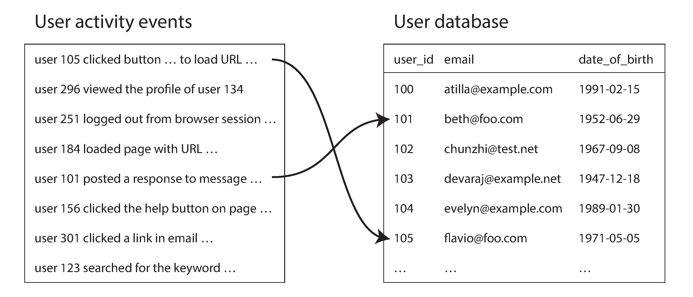
Figure 11-2 A join between a log of user activity events and a database of user profiles.

If you want to perform an analysis of the activity events that takes into account information from the user database (for example, find out whether certain pages are more popular with younger or older users, using the date of birth field in the user profile), you need to compute a join between these two tables. How would you compute that join, assuming both tables are so large that they have to be sharded?

You can use the fact that in MapReduce, the shuffle brings together all the key-value pairs with the same key to the same reducer, no matter which shard they were on originally. Here, the user ID can serve as the key. You can therefore write a mapper that goes over the user activity events, and emits page view URLs keyed by user ID, as illustrated in Figure 11-3. Another mapper goes over the user database row by row, extracting the user ID as the key and the user’s date of birth as the value.

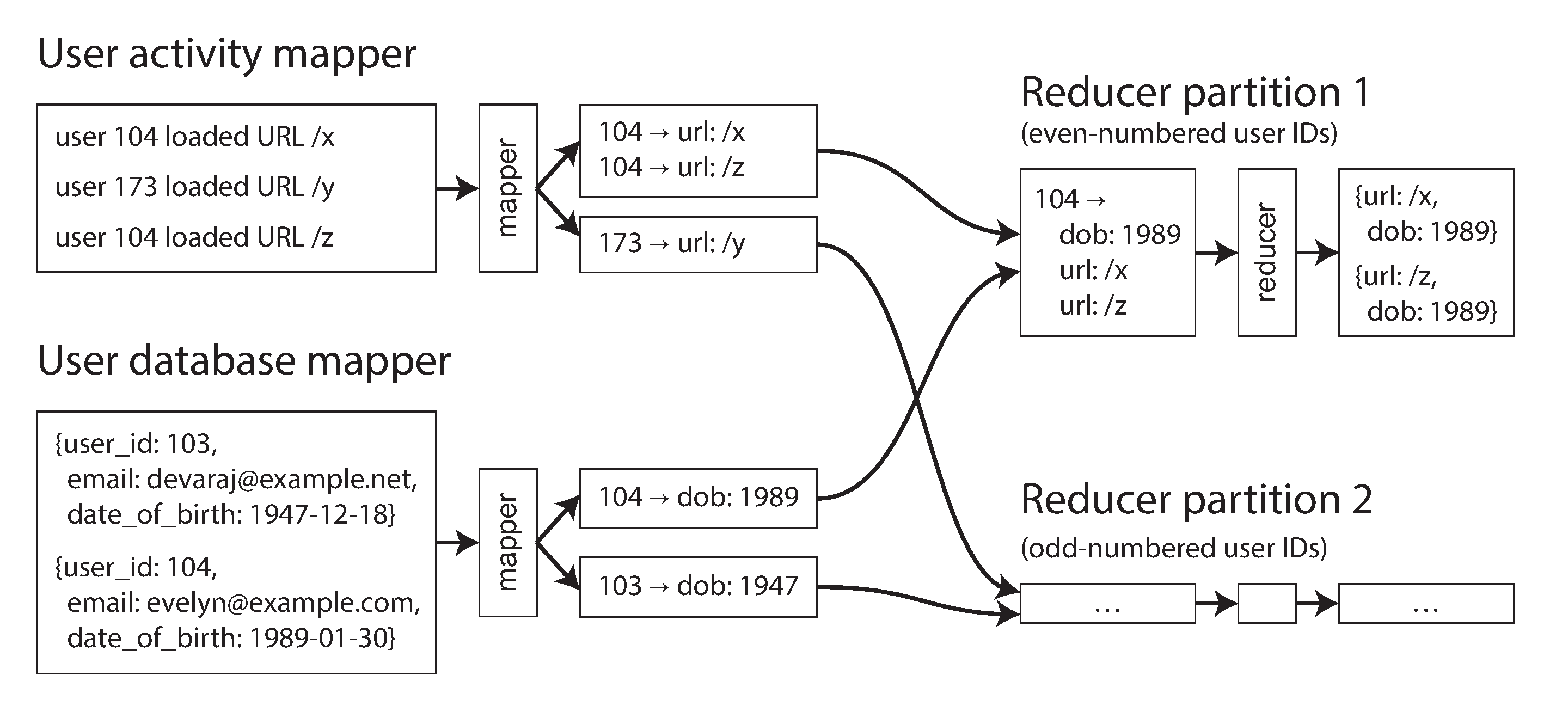
Figure 11-3 A sort-merge join on user ID. If the input datasets are sharded into multiple files, each could be processed with multiple mappers in parallel.

The shuffle then ensures that a reducer function can access a particular user’s date of birth and all of that user’s page view events at the same time. The MapReduce job can even arrange the records to be sorted such that the reducer always sees the record from the user database first, followed by the activity events in timestamp order—this technique is known as a secondary sort ²⁵.

The reducer can then perform the actual join logic easily. The first value is expected to be the date of birth, which the reducer stores in a local variable. It then iterates over the activity events with the same user ID, outputting each viewed URL along with the viewer’s date of birth. Since the reducer processes all of the records for a particular user ID in one go, it only needs to keep one user record in memory at any one time, and it never needs to make any requests over the network. This algorithm is known as a sort-merge join, since mapper output is sorted by key, and the reducers then merge together the sorted lists of records from both sides of the join.

The next MapReduce job in the workflow can then calculate the distribution of viewer ages for each URL. To do so, the job would first shuffle the data using the URL as key. Once sorted, the reducers would then iterate over all the page views (with viewer birth date) for a single URL, keep a counter for the number of views by each age group, and increment the appropriate counter for each page view. This way you can implement a group by operation and aggregation.

Query languages

Over the years, execution engines for distributed batch processing have matured. By now, the infrastructure has become robust enough to store and process many petabytes of data on clusters of over 10,000 machines. As the problem of physically operating batch processes at such scale has been considered more or less solved, attention has turned to improving the programming model.

MapReduce, dataflow engines, and cloud data warehouses have all embraced SQL as the lingua franca for batch processing. It’s a natural fit: legacy data warehouses used SQL, data analytics and ETL tools already support SQL, and all developers and analysts know it.

Besides the obvious advantage of requiring less code than handwritten MapReduce jobs, these query language interfaces also allow interactive use, in which you write analytical queries and run them from a terminal or GUI. This style of interactive querying is an efficient and natural way for business analytics, product managers, sales and finance teams, and others to explore data in a batch processing environment. Though not a classic form of batch processing, SQL support has made exploratory queries suitable for distributed batch processing systems.

High-level query languages not only make the humans using the system more productive, but they also improve the job execution efficiency at a machine level. As we saw in “Cloud Data Warehouses”, query engines are responsible for converting SQL queries into batch jobs to be executed in a cluster. This translation step from query to syntax tree to physical operators allows the engine to optimize queries. Query engines such as Hive, Trino, Spark, and Flink have cost-based query optimizers that can analyze the properties of join inputs and automatically decide which algorithm would be most suitable for the task at hand. Optimizers might even change the order of joins so that the amount of intermediate state is minimized ¹⁹, ²⁶, ²⁷, ²⁸.

While SQL is the most popular general-purpose batch processing query language, other languages remain in use for niche use cases. Apache Pig was a language based on relational operators that allowed data pipelines to be specified step by step, rather than as one big SQL query. DataFrames (see next section) have similar characteristics, and Morel is a more modern language influenced by Pig. Other users have adopted JSON query languages such as jq, JMESPath, or JsonPath.

In “Graph-Like Data Models” we discussed using graphs for modeling data, and using graph query languages to traverse the edges and vertices in a graph. Many graph processing frameworks also support batch computation through query languages such as Apache TinkerPop’s Gremlin. We will look at graph processing use cases in more detail in “Batch Use Cases”.

BATCH PROCESSING AND CLOUD DATA WAREHOUSES CONVERGE

Historically, data warehouses ran on specialized hardware appliances, and provided SQL analytics queries over relational data. In contrast, batch processing frameworks like MapReduce set out to provide greater scalability and greater flexibility by supporting processing logic written in a general-purpose programming language, allowing it to read and write arbitrary data formats.

Over time, the two have become much more similar. Modern batch processing frameworks now support SQL as a language for writing batch jobs, and they achieve good performance on relational queries by using columnar storage formats such as Parquet and optimized query execution engines (see “Query Execution: Compilation and Vectorization”). Meanwhile, data warehouses have grown more scalable by moving to the cloud (see “Cloud Data Warehouses”), and implementing many of the same scheduling, fault tolerance, and shuffling techniques that distributed batch frameworks do. Many use distributed filesystems as well.

Just as batch processing systems adopted SQL as a processing model, cloud warehouses have adopted alternative processing models such as DataFrames as well (discussed in the next section). For example, Google Cloud BigQuery offers a BigQuery DataFrames library and Snowflake’s Snowpark integrates with Pandas. Batch processing workflow orchestrators such as Airflow, Prefect, and Dagster also integrate with cloud warehouses.

Not all batch jobs are easily expressed in SQL, though. Iterative graph algorithms such as PageRank, complex machine learning, and many other tasks are difficult to express in SQL. AI data processing, which includes non-relational and multi-modal data such as images, video, and audio, can also be difficult to do in SQL.

Moreover, cloud data warehouses struggle with certain workloads. Row-by-row computation is less efficient when using column-oriented storage formats. Alternative warehouse APIs or a batch processing system are preferable in such cases. Cloud data warehouses also tend to be more expensive than other batch processing systems. It can be more cost-efficient to run large jobs in batch processing systems such as Spark or Flink instead.

Ultimately, the decision between processing data in batch systems or data warehouses comes down to factors such as cost, convenience, ease of implementation, availability, and so on. Most large enterprises have many data processing systems, which give them flexibility in this decision. Smaller companies often get by with just one.

DataFrames

As data scientists and statisticians began using distributed batch processing frameworks for machine learning use cases, they found existing processing models cumbersome, as they were used to working with the DataFrame data model found in R and Pandas (see “DataFrames, Matrices, and Arrays”). A DataFrame is similar to a table in a relational database: it is a collection of rows, and all the values in the same column have the same type. Instead of writing one big SQL query, users call functions corresponding to relational operators to perform filters, joins, sorting, group by, and other operations.

Originally, DataFrame manipulation typically occurred locally, in memory. Consequently, DataFrames were limited to datasets that fit on a single machine. Data scientists wanted to interact with the large datasets found in batch processing environments using the DataFrame APIs they were used to. Distributed data processing frameworks such as Spark, Flink, and Daft have adopted DataFrame APIs to meet this need. On the other hand, local DataFrames are usually indexed and ordered while distributed DataFrames are generally not ²⁹. This can lead to performance surprises when migrating to batch frameworks.

DataFrame APIs appear similar to dataflow APIs, but implementations vary. While Pandas executes operations immediately when the DataFrame methods are called, Apache Spark first translates all the DataFrame API calls into a query plan and runs query optimization before executing the workflow on top of its distributed dataflow engine. This allows it to improve performance.

Frameworks such as Daft even support both client and server-side computation. Smaller, in-memory operations are executed on the client while larger datasets and computation are executed on the server. Columnar storage formats such as Apache Arrow offer a unified data model that both client and server-side execution engines can share.

Batch Use Cases

Now that we’ve seen how batch processing works, let’s see how it is applied to a range of different applications. Batch jobs are excellent for processing large datasets in bulk, but they aren’t good for low latency use cases. Consequently, you’ll find batch jobs wherever there’s a lot of data and data freshness isn’t important. This might sound limiting, but it turns out that the a significant amount of data processing fits this model:

Accounting and inventory reconciliation, where companies verify that transactions line up with their bank accounts and inventory, are often done in batch ³⁰.
In manufacturing, demand forecasting is computed in periodic batch jobs ³¹.
Ecommerce, media, and social media companies train their recommendation models using batch jobs ³², ³³.
Many financial systems are batch-based, as well. For example, the United States’s banking network runs almost entirely on batch jobs ³⁴.

In the following sections, we’ll discuss some of the batch processing use cases you’ll find in nearly every industry.

Extract–Transform–Load (ETL)

“Data Warehousing” introduced the idea of ETL and ELT, where a data processing pipeline extracts data from a production database, transforms it, and loads results into a downstream system (we’ll use “ETL” in this section to represent both ETL and ELT workloads). Batch jobs are often used for such workloads, especially when the downstream system is a data warehouse.

The parallel nature of batch jobs makes them a great fit for data transformation. Much of data transformation involves “embarrassingly parallel” workloads. Filtering data, projecting fields, and many other common data warehouse transformations can all be done in parallel.

Batch processing environments also come with robust workflow schedulers, which make it easy to schedule, orchestrate, and debug ETL data pipeline jobs. When a failure occurs, schedulers often retry jobs to mitigate transient issues that might occur. A job that fails repeatedly will be marked as failed, which helps developers easily see which job in their data pipeline stopped working. Schedulers like Airflow even come with built-in source, sink, and query operators for MySQL, PostgreSQL, Snowflake, Spark, Flink, and dozens of other popular systems. A tight integration between schedulers and data processing systems simplifies data integration.

We’ve also seen that batch jobs are easy to troubleshoot and fix when things go awry. This feature is invaluable when debugging data pipelines. Failed files can be easily inspected to see what went wrong, and ETL batch jobs can be fixed and re-run. For example, an input file might no longer contain a field that a transformation batch job intends to use. Data engineers will see that the field is missing, and update the transformation logic or the job that produced the input.

Data pipelines used to be managed by a single data engineering team, as it was considered unfair to ask other teams working on product features to write and manage complex batch data pipelines. Recently, improvements in batch processing models and metadata management have made it much easier for engineers across an organization to contribute to and manage their own data pipelines. Data mesh ³⁵, ³⁶, data contract ³⁷, and data fabric ³⁸ practices provide standards and tools to help teams safely publish their data for consumption by anybody in the organization.

Data pipelines and analytic queries have begun to share not only processing models, but execution engines as well. Many batch ETL jobs now run on the same systems as the analytic queries that read their output. It is not uncommon to see data pipeline transformations and analytic queries both run as SparkSQL, Trino, or DuckDB queries. Such an architecture further blurs the line between application engineering, data engineering, analytics engineering, and business analysis.

Analytics

In “Operational Versus Analytical Systems”, we saw that analytic queries (OLAP) often scan over a large number of records, performing groupings and aggregations. It is possible to run such workloads in a batch processing system, alongside other batch processing workloads. Analysts write SQL queries that execute atop a query engine, which reads and writes from a distributed file system or object store. Table metadata such as table to file mappings, names, and types are managed with table formats such as Apache Iceberg and catalogs such as Unity (see “Cloud Data Warehouses”). This architecture is known as a data lakehouse ³⁹.

As with ETL, improvements in SQL query interfaces mean many organizations now use batch frameworks such as Spark for analytics. Such query patterns come in two styles:

Pre-aggregation queries, where data is rolled up into OLAP cubes or data marts to speed up queries (see “Materialized Views and Data Cubes”). Pre-aggregated data is queried in the warehouse or pushed to purpose-built realtime OLAP systems such as Apache Druid or Apache Pinot. Pre-aggregation normally takes place at a scheduled interval. The workflow schedulers discussed in “Scheduling Workflows” are used to manage these workloads.
Ad hoc queries that users run to answer specific business questions, investigate user behavior, debug operational issues, and much more. Response times are important for this use case. Analysts run queries iteratively as they get responses and learn more about the data they’re investigating. Batch processing frameworks with fast query execution help reduce waiting times for analysts.

SQL support enables batch processing frameworks to integrate with spreadsheets and data visualization tools such as Tableau, Power BI, Looker, and Apache Superset. For example, Tableau offers SparkSQL and Presto connectors, while Apache Superset supports Trino, Hive, Spark SQL, Presto, and many other systems that ultimately execute batch jobs to query data.

Machine Learning

Machine learning (ML) makes frequent use of batch processing. Data scientists, ML engineers, and AI engineers use batch processing frameworks to investigate data patterns, transform data, and train machine learning models. Common uses include:

Feature engineering: Raw data is filtered and transformed into data that models can be trained on. Predictive models often need numeric data, so engineers must transform other forms of data (such as text or discrete values) into the required format.
Model training: The training data is the input to the batch process, and the weights of the trained model are the output.
Batch inference: A trained model can then be used to make predictions in bulk if datasets are large and realtime results are not required. This includes evaluating the model’s predictions on a test dataset.

Batch processing frameworks provide tools explicitly for these use cases. For example, Apache Spark’s MLlib and Apache Flink’s FlinkML come with a wide variety of feature engineering tools, statistical functions, and classifiers.

Machine learning applications such as recommendation engines and ranking systems also make heavy use of graph processing (see “Graph-Like Data Models”). Many graph algorithms are expressed by traversing one edge at a time, joining one vertex with an adjacent vertex in order to propagate some information, and repeating until some condition is met—for example, until there are no more edges to follow, or until some metric converges.

The bulk synchronous parallel (BSP) model of computation ⁴⁰ has become popular for batch processing graphs. Among others, it is implemented by Apache Giraph ²⁰, Spark’s GraphX API, and Flink’s Gelly API ⁴¹. It is also known as the Pregel model, as Google’s Pregel paper popularized this approach for processing graphs ⁴².

Batch processing is also an integral part of large language model (LLM) data preparation and training. Raw text input data such as websites typically reside in a DFS or object store. This data must be pre-processed to make it suitable for training. Pre-processing steps that are well-suited for batch processing frameworks include:

Plain text must be extracted from HTML and malformed text must be fixed.
Low quality, irrelevant, and duplicate documents must be detected and removed.
Text must be tokenized (split into words) and converted into embeddings, which are numeric representations of each word.

Batch processing frameworks such as Kubeflow, Flyte, and Ray are purpose-built for such workloads. OpenAI uses Ray as part of its ChatGPT training process, for example ⁴³. These frameworks have built-in integrations for LLM and AI libraries such as PyTorch, Tensorflow, XGBoost, and many others. They also offer built-in support for feature engineering, model training, batch inference, and fine tuning (adjusting a foundational model for specific use cases).

Finally, data scientists often experiment with data in interactive notebooks such as Jupyter or Hex. Notebooks are made up of cells, which are small chunks of markdown, Python, or SQL. Cells are executed sequentially to produce spreadsheets, graphs, or data. Many notebooks use batch processing via DataFrame APIs or query such systems using SQL.

Serving Derived Data

Batch jobs are often used to build pre-computed or derived datasets such as product recommendations, user-facing reports, and features for machine learning models. These datasets are typically served from a production database, key-value store, or search engine. Regardless of the system used, the pre-computed data needs to make its way from the batch processor’s distributed filesystem or object store back into the database that’s serving live traffic.

The most obvious choice might be to use the client library for your favorite database directly within a batch job, and to write directly to the database server, one record at a time. This will work (assuming your firewall rules allow direct access from your batch processing environment to your production databases), but it is a bad idea for several reasons:

Making a network request for every single record is orders of magnitude slower than the normal throughput of a batch task. Even if the client library supports batching, performance is likely to be poor.
Batch processing frameworks often run many tasks in parallel. If all the tasks concurrently write to the same output database, with a rate expected of a batch process, that database can easily be overwhelmed, and its performance for queries is likely to suffer. This can in turn cause operational problems in other parts of the system ⁴⁴.
Normally, batch jobs provide a clean all-or-nothing guarantee for job output: if a job succeeds, the result is the output of running every task exactly once, even if some tasks failed and had to be retried along the way; if the entire job fails, no output is produced. However, writing to an external system from inside a job produces externally visible side effects that cannot be hidden in this way. Thus, you have to worry about the results from partially completed jobs being visible to other systems. If a task fails and is restarted, it may duplicate output from the failed execution.

A better solution is to have batch jobs push pre-computed datasets to streams such as Kafka topics, which we discuss further in Chapter 12. Search engines like Elasticsearch, realtime OLAP systems like Apache Pinot and Apache Druid, derived datastores like Venice ⁴⁵, and cloud data warehouses like ClickHouse all have the built-in ability to ingest data from Kafka into their systems. Pushing data through a streaming systems fixes a few of the problems we discussed above:

Streaming systems are optimized for sequential writes, which make them better suited for the bulk write workload of a batch job.
Streaming systems can also act as a buffer between the batch job and the production databases. Downstream systems can throttle their read rate to ensure they can continue to comfortably serve production traffic.
The output of a single batch job can be consumed by multiple downstream systems.
Streaming systems can serve as a security boundary between batch processing environments and production networks: they can be deployed in a so-called DMZ (demilitarized zone) network that sits between the batch processing network and production network.

Pushing data through streams doesn’t inherently solve the all-or-nothing guarantee issue we discussed above. To make this work, batch jobs must send a notification to downstream systems that their job is complete and the data can now be served. Consumers of the stream need to be able to keep data they receive invisible to queries, like an uncommitted transaction with read committed isolation (see “Read Committed”), until they are notified that it is complete.

Another pattern that is more common when bootstrapping databases is to build a brand-new database inside the batch job and bulk load those files directly into the database from a distributed filesystem, object store, or local filesystem. Many data systems offer bulk import tools such as TiDB’s Lightning tool, or Apache Pinot’s and Apache Druid’s Hadoop import jobs. RocksDB also offers an API to bulk import SSTs from batch jobs.

Building databases in batch and bulk importing the data is very fast, and makes it easier for systems to atomically switch between dataset versions. On the other hand, it can be challenging to incrementally update datasets from batch jobs that build brand-new databases. It’s common to take a hybrid approach in situations where both bootstrapping and incremental loads are needed. Venice, for example, supports hybrid stores that allow for batch row-based updates and full dataset swaps.

Summary

In this chapter, we explored the design and implementation of batch processing systems. We began with the classic Unix toolchain (awk, sort, uniq, etc.), to illustrate fundamental batch processing primitives such as sorting and counting.

We then scaled up to distributed batch processing systems. We saw that batch-style I/O processes immutable, bounded input datasets to produce output data, allowing reruns and debugging without side effects. To process files, we saw that batch frameworks have three main components: an orchestration layer that determines where and when jobs run, a storage layer to persist data, and a computation layer that processes the actual data.

We looked at how distributed filesystems and object stores manage large files through block-based replication, caching, and metadata services, and how modern batch frameworks interact with these systems using pluggable APIs. We also discussed how orchestrators schedule tasks, allocate resources, and handle faults in large clusters. We also compared job orchestrators that schedule jobs with workflow orchestrators that manage the lifecycle of a collection of jobs that run in a dependency graph.

We surveyed batch processing models, starting with MapReduce and its canonical map and reduce functions. Next, we turned to dataflow engines like Spark and Flink, which offer simpler-to-use dataflow APIs and better performance. To understand how batch jobs scale, we covered the shuffle algorithm, a foundational operation that enables grouping, joining, and aggregation.

As batch systems matured, focus shifted to usability. You learned about high-level query languages like SQL and DataFrame APIs, which make batch jobs more accessible and easier to optimize. Query optimizers translate declarative queries into efficient execution plans.

We finished the chapter with common batch processing use cases:

ETL pipelines, which extract, transform, and load data between different systems using scheduled workflows;
Analytics, where batch jobs support both pre-aggregated dashboards and ad hoc queries;
Machine learning, where batch jobs prepare and process large training datasets;
Populating production-facing systems from batch outputs, often via streams or bulk loading tools, in order to serve the derived data to users.

In the next chapter, we will turn to stream processing, in which the input is unbounded—that is, you still have a job, but its inputs are never-ending streams of data. In this case, a job is never complete, because at any time there may still be more work coming in. We shall see that stream and batch processing are similar in some respects, but the assumption of unbounded streams also changes a lot about how we build systems.

Footnotes

References

Nathan Marz. How to Beat the CAP Theorem. nathanmarz.com, October 2011. Archived at perma.cc/4BS9-R9A4 ↩︎
Molly Bartlett Dishman and Martin Fowler. Agile Architecture. At O’Reilly Software Architecture Conference, March 2015. ↩︎
Jeffrey Dean and Sanjay Ghemawat. MapReduce: Simplified Data Processing on Large Clusters. At 6th USENIX Symposium on Operating System Design and Implementation (OSDI), December 2004. ↩︎ ↩︎
Shivnath Babu and Herodotos Herodotou. Massively Parallel Databases and MapReduce Systems. Foundations and Trends in Databases, volume 5, issue 1, pages 1–104, November 2013. doi:10.1561/1900000036 ↩︎
David J. DeWitt and Michael Stonebraker. MapReduce: A Major Step Backwards. Originally published at databasecolumn.vertica.com, January 2008. Archived at perma.cc/U8PA-K48V ↩︎
Henry Robinson. The Elephant Was a Trojan Horse: On the Death of Map-Reduce at Google. the-paper-trail.org, June 2014. Archived at perma.cc/9FEM-X787 ↩︎
Urs Hölzle. R.I.P. MapReduce. After having served us well since 2003, today we removed the remaining internal codebase for good. twitter.com, September 2019. Archived at perma.cc/B34T-LLY7 ↩︎
Adam Drake. Command-Line Tools Can Be 235x Faster than Your Hadoop Cluster. aadrake.com, January 2014. Archived at perma.cc/87SP-ZMCY ↩︎
sort: Sort text files. GNU Coreutils 9.7 Documentation, Free Software Foundation, Inc., 2025. ↩︎
Michael Ovsiannikov, Silvius Rus, Damian Reeves, Paul Sutter, Sriram Rao, and Jim Kelly. The Quantcast File System. Proceedings of the VLDB Endowment, volume 6, issue 11, pages 1092–1101, August 2013. doi:10.14778/2536222.2536234 ↩︎
Andrew Wang, Zhe Zhang, Kai Zheng, Uma Maheswara G., and Vinayakumar B. Introduction to HDFS Erasure Coding in Apache Hadoop. blog.cloudera.com, September 2015. Archived at archive.org ↩︎
Andy Warfield. Building and operating a pretty big storage system called S3. allthingsdistributed.com, July 2023. Archived at perma.cc/7LPK-TP7V ↩︎
Vinod Kumar Vavilapalli, Arun C. Murthy, Chris Douglas, Sharad Agarwal, Mahadev Konar, Robert Evans, Thomas Graves, Jason Lowe, Hitesh Shah, Siddharth Seth, Bikas Saha, Carlo Curino, Owen O’Malley, Sanjay Radia, Benjamin Reed, and Eric Baldeschwieler. Apache Hadoop YARN: Yet Another Resource Negotiator. At 4th Annual Symposium on Cloud Computing (SoCC), October 2013. doi:10.1145/2523616.2523633 ↩︎
Richard M. Karp. Reducibility Among Combinatorial Problems. Complexity of Computer Computations. The IBM Research Symposia Series. Springer, 1972. doi:10.1007/978-1-4684-2001-2_9 ↩︎
J. D. Ullman. NP-Complete Scheduling Problems. Journal of Computer and System Sciences, volume 10, issue 3, June 1975. doi:10.1016/S0022-0000(75)80008-0 ↩︎
Gilad David Maayan. The complete guide to spot instances on AWS, Azure and GCP. datacenterdynamics.com, March 2021. Archived at archive.org ↩︎
Abhishek Verma, Luis Pedrosa, Madhukar Korupolu, David Oppenheimer, Eric Tune, and John Wilkes. Large-Scale Cluster Management at Google with Borg. At 10th European Conference on Computer Systems (EuroSys), April 2015. doi:10.1145/2741948.2741964 ↩︎
Matei Zaharia, Mosharaf Chowdhury, Tathagata Das, Ankur Dave, Justin Ma, Murphy McCauley, Michael J. Franklin, Scott Shenker, and Ion Stoica. Resilient Distributed Datasets: A Fault-Tolerant Abstraction for In-Memory Cluster Computing. At 9th USENIX Symposium on Networked Systems Design and Implementation (NSDI), April 2012. ↩︎ ↩︎
Paris Carbone, Stephan Ewen, Seif Haridi, Asterios Katsifodimos, Volker Markl, and Kostas Tzoumas. Apache Flink™: Stream and Batch Processing in a Single Engine. Bulletin of the IEEE Computer Society Technical Committee on Data Engineering, volume 38, issue 4, December 2015. Archived at perma.cc/G3N3-BKX5 ↩︎ ↩︎ ↩︎
Mark Grover, Ted Malaska, Jonathan Seidman, and Gwen Shapira. Hadoop Application Architectures. O’Reilly Media, 2015. ISBN: 978-1-491-90004-8 ↩︎ ↩︎
Jules S. Damji, Brooke Wenig, Tathagata Das, and Denny Lee. Learning Spark, 2nd Edition. O’Reilly Media, 2020. ISBN: 978-1492050049 ↩︎
Michael Isard, Mihai Budiu, Yuan Yu, Andrew Birrell, and Dennis Fetterly. Dryad: Distributed Data-Parallel Programs from Sequential Building Blocks. At 2nd European Conference on Computer Systems (EuroSys), March 2007. doi:10.1145/1272996.1273005 ↩︎
Daniel Warneke and Odej Kao. Nephele: Efficient Parallel Data Processing in the Cloud. At 2nd Workshop on Many-Task Computing on Grids and Supercomputers (MTAGS), November 2009. doi:10.1145/1646468.1646476 ↩︎
Hossein Ahmadi. In-memory query execution in Google BigQuery. cloud.google.com, August 2016. Archived at perma.cc/DGG2-FL9W ↩︎ ↩︎
Tom White. Hadoop: The Definitive Guide, 4th edition. O’Reilly Media, 2015. ISBN: 978-1-491-90163-2 ↩︎ ↩︎
Fabian Hüske. Peeking into Apache Flink’s Engine Room. flink.apache.org, March 2015. Archived at perma.cc/44BW-ALJX ↩︎
Mostafa Mokhtar. Hive 0.14 Cost Based Optimizer (CBO) Technical Overview. hortonworks.com, March 2015. Archived on archive.org ↩︎
Michael Armbrust, Reynold S. Xin, Cheng Lian, Yin Huai, Davies Liu, Joseph K. Bradley, Xiangrui Meng, Tomer Kaftan, Michael J. Franklin, Ali Ghodsi, and Matei Zaharia. Spark SQL: Relational Data Processing in Spark. At ACM International Conference on Management of Data (SIGMOD), June 2015. doi:10.1145/2723372.2742797 ↩︎
Kaya Kupferschmidt. Spark vs Pandas, part 2 – Spark. towardsdatascience.com, October 2020. Archived at perma.cc/5BRK-G4N5 ↩︎
Ammar Chalifah. Tracking payments at scale. bolt.eu.com, June 2025. Archived at perma.cc/Q4KX-8K3J ↩︎
Nafi Ahmet Turgut, Hamza Akyıldız, Hasan Burak Yel, Mehmet İkbal Özmen, Mutlu Polatcan, Pinar Baki, and Esra Kayabali. Demand forecasting at Getir built with Amazon Forecast. aws.amazon.com.com, May 2023. Archived at perma.cc/H3H6-GNL7 ↩︎
Jason (Siyu) Zhu. Enhancing homepage feed relevance by harnessing the power of large corpus sparse ID embeddings. linkedin.com, August 2023. Archived at archive.org ↩︎
Avery Ching, Sital Kedia, and Shuojie Wang. Apache Spark @Scale: A 60 TB+ production use case. engineering.fb.com, August 2016. Archived at perma.cc/F7R5-YFAV ↩︎
Edward Kim. How ACH works: A developer perspective — Part 1. engineering.gusto.com, April 2014. Archived at perma.cc/F67P-VBLK ↩︎
Zhamak Dehghani. How to Move Beyond a Monolithic Data Lake to a Distributed Data Mesh. martinfowler.com, May 2019. Archived at perma.cc/LN2L-L4VC ↩︎
Chris Riccomini. What the Heck is a Data Mesh?! cnr.sh, June 2021. Archived at perma.cc/NEJ2-BAX3 ↩︎
Chad Sanderson, Mark Freeman, B. E. Schmidt. Data Contracts. O’Reilly Media, 2025. ISBN: 9781098157623 ↩︎
Daniel Abadi. Data Fabric vs. Data Mesh: What’s the Difference? starburst.io, November 2021. Archived at perma.cc/RSK3-HXDK ↩︎
Michael Armbrust, Ali Ghodsi, Reynold Xin, and Matei Zaharia. Lakehouse: A New Generation of Open Platforms that Unify Data Warehousing and Advanced Analytics. At 11th Annual Conference on Innovative Data Systems Research (CIDR), January 2021. ↩︎
Leslie G. Valiant. A Bridging Model for Parallel Computation. Communications of the ACM, volume 33, issue 8, pages 103–111, August 1990. doi:10.1145/79173.79181 ↩︎
Stephan Ewen, Kostas Tzoumas, Moritz Kaufmann, and Volker Markl. Spinning Fast Iterative Data Flows. Proceedings of the VLDB Endowment, volume 5, issue 11, pages 1268-1279, July 2012. doi:10.14778/2350229.2350245 ↩︎
Grzegorz Malewicz, Matthew H. Austern, Aart J. C. Bik, James C. Dehnert, Ilan Horn, Naty Leiser, and Grzegorz Czajkowski. Pregel: A System for Large-Scale Graph Processing. At ACM International Conference on Management of Data (SIGMOD), June 2010. doi:10.1145/1807167.1807184 ↩︎
Richard MacManus. OpenAI Chats about Scaling LLMs at Anyscale’s Ray Summit. thenewstack.io, September 2023. Archived at perma.cc/YJD6-KUXU ↩︎
Jay Kreps. Why Local State is a Fundamental Primitive in Stream Processing. oreilly.com, July 2014. Archived at perma.cc/P8HU-R5LA ↩︎
Félix GV. Open Sourcing Venice – LinkedIn’s Derived Data Platform. linkedin.com, September 2022. Archived at archive.org ↩︎

12. Stream Processing

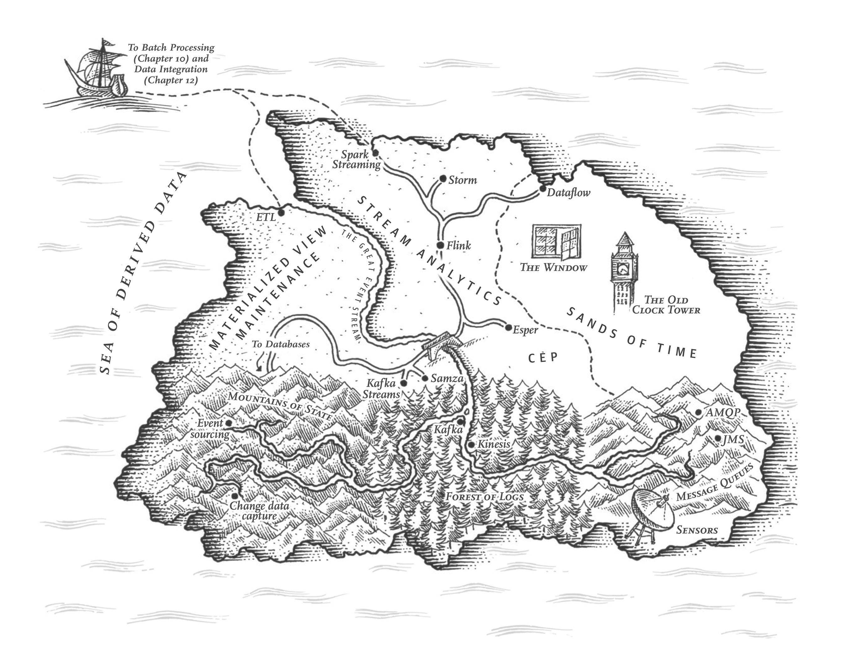
A complex system that works is invariably found to have evolved from a simple system that works. The inverse proposition also appears to be true: A complex system designed from scratch never works and cannot be made to work.

John Gall, Systemantics (1975)

A NOTE FOR EARLY RELEASE READERS

This will be the 12th chapter of the final book. The GitHub repo for this book is https://github.com/ept/ddia2-feedback.

If you’d like to be actively involved in reviewing and commenting on this draft, please reach out on GitHub.

In Chapter 11 we discussed batch processing—techniques that read a set of files as input and produce a new set of output files. The output is a form of derived data; that is, a dataset that can be recreated by running the batch process again if necessary. We saw how this simple but powerful idea can be used to create search indexes, recommendation systems, analytics, and more.

However, one big assumption remained throughout Chapter 11: namely, that the input is bounded—i.e., of a known and finite size—so the batch process knows when it has finished reading its input. For example, the sorting operation that is central to MapReduce must read its entire input before it can start producing output: it could happen that the very last input record is the one with the lowest key, and thus needs to be the very first output record, so starting the output early is not an option.

In reality, a lot of data is unbounded because it arrives gradually over time: your users produced data yesterday and today, and they will continue to produce more data tomorrow. Unless you go out of business, this process never ends, and so the dataset is never “complete” in any meaningful way ¹. Thus, batch processors must artificially divide the data into chunks of fixed duration: for example, processing a day’s worth of data at the end of every day, or processing an hour’s worth of data at the end of every hour.

The problem with daily batch processes is that changes in the input are only reflected in the output a day later, which is too slow for many impatient users. To reduce the delay, we can run the processing more frequently—say, processing a second’s worth of data at the end of every second—or even continuously, abandoning the fixed time slices entirely and simply processing every event as it happens. That is the idea behind stream processing.

In general, a “stream” refers to data that is incrementally made available over time. The concept appears in many places: in the stdin and stdout of Unix, programming languages (lazy lists) ², filesystem APIs (such as Java’s FileInputStream), TCP connections, delivering audio and video over the internet, and so on.

In this chapter we will look at event streams as a data management mechanism: the unbounded, incrementally processed counterpart to the batch data we saw in the last chapter. We will first discuss how streams are represented, stored, and transmitted over a network. In “Databases and Streams” we will investigate the relationship between streams and databases. And finally, in “Processing Streams” we will explore approaches and tools for processing those streams continually, and ways that they can be used to build applications.

Transmitting Event Streams

In the batch processing world, the inputs and outputs of a job are files (perhaps on a distributed filesystem). What does the streaming equivalent look like?

When the input is a file (a sequence of bytes), the first processing step is usually to parse it into a sequence of records. In a stream processing context, a record is more commonly known as an event, but it is essentially the same thing: a small, self-contained, immutable object containing the details of something that happened at some point in time. An event usually contains a timestamp indicating when it happened according to a time-of-day clock (see “Monotonic Versus Time-of-Day Clocks”).

For example, the thing that happened might be an action that a user took, such as viewing a page or making a purchase. It might also originate from a machine, such as a periodic measurement from a temperature sensor, or a CPU utilization metric. In the example of “Batch Processing with Unix Tools”, each line of the web server log is an event.

An event may be encoded as a text string, or JSON, or perhaps in some binary form, as discussed in Chapter 5. This encoding allows you to store an event, for example by appending it to a file, inserting it into a relational table, or writing it to a document database. It also allows you to send the event over the network to another node in order to process it.

In batch processing, a file is written once and then potentially read by multiple jobs. Analogously, in streaming terminology, an event is generated once by a producer (also known as a publisher or sender), and then potentially processed by multiple consumers (subscribers or recipients) ³. In a filesystem, a filename identifies a set of related records; in a streaming system, related events are usually grouped together into a topic or stream.

In principle, a file or database is sufficient to connect producers and consumers: a producer writes every event that it generates to the datastore, and each consumer periodically polls the datastore to check for events that have appeared since it last ran. This is essentially what a batch process does when it processes a day’s worth of data at the end of every day.

However, when moving toward continual processing with low delays, polling becomes expensive if the datastore is not designed for this kind of usage. The more often you poll, the lower the percentage of requests that return new events, and thus the higher the overheads become. Instead, it is better for consumers to be notified when new events appear.

Databases have traditionally not supported this kind of notification mechanism very well: relational databases commonly have triggers, which can react to a change (e.g., a row being inserted into a table), but they are very limited in what they can do and have been somewhat of an afterthought in database design ⁴. Instead, specialized tools have been developed for the purpose of delivering event notifications.

Messaging Systems

A common approach for notifying consumers about new events is to use a messaging system: a producer sends a message containing the event, which is then pushed to consumers. We touched on these systems previously in “Event-Driven Architectures”, but we will now go into more detail.

A direct communication channel like a Unix pipe or TCP connection between producer and consumer would be a simple way of implementing a messaging system. However, most messaging systems expand on this basic model. In particular, Unix pipes and TCP connect exactly one sender with one recipient, whereas a messaging system allows multiple producer nodes to send messages to the same topic and allows multiple consumer nodes to receive messages in a topic.

Within this publish/subscribe model, different systems take a wide range of approaches, and there is no one right answer for all purposes. To differentiate the systems, it is particularly helpful to ask the following two questions:

What happens if the producers send messages faster than the consumers can process them? Broadly speaking, there are three options: the system can drop messages, buffer messages in a queue, or apply backpressure (also known as flow control; i.e., blocking the producer from sending more messages). For example, Unix pipes and TCP use backpressure: they have a small fixed-size buffer, and if it fills up, the sender is blocked until the recipient takes data out of the buffer (see “Network congestion and queueing”).

If messages are buffered in a queue, it is important to understand what happens as that queue grows. Does the system crash if the queue no longer fits in memory, or does it write messages to disk? In the latter case, how does the disk access affect the performance of the messaging system ⁵, and what happens when the disk fills up ⁶?
What happens if nodes crash or temporarily go offline—are any messages lost? As with databases, durability may require some combination of writing to disk and/or replication (see the sidebar “Replication and Durability”), which has a cost. If you can afford to sometimes lose messages, you can probably get higher throughput and lower latency on the same hardware.

Whether message loss is acceptable depends very much on the application. For example, with sensor readings and metrics that are transmitted periodically, an occasional missing data point is perhaps not important, since an updated value will be sent a short time later anyway. However, beware that if a large number of messages are dropped, it may not be immediately apparent that the metrics are incorrect ⁷. If you are counting events, it is more important that they are delivered reliably, since every lost message means incorrect counters.

A nice property of the batch processing systems we explored in Chapter 11 is that they provide a strong reliability guarantee: failed tasks are automatically retried, and partial output from failed tasks is automatically discarded. This means the output is the same as if no failures had occurred, which helps simplify the programming model. Later in this chapter we will examine how we can provide similar guarantees in a streaming context.

Direct messaging from producers to consumers

A number of messaging systems use direct network communication between producers and consumers without going via intermediary nodes:

UDP multicast is widely used in the financial industry for streams such as stock market feeds, where low latency is important ⁸. Although UDP itself is unreliable, application-level protocols can recover lost packets (the producer must remember packets it has sent so that it can retransmit them on demand).
Brokerless messaging libraries such as ZeroMQ and nanomsg take a similar approach, implementing publish/subscribe messaging over TCP or IP multicast.
Some metrics collection agents, such as StatsD ⁹ use unreliable UDP messaging to collect metrics from all machines on the network and monitor them. (In the StatsD protocol, counter metrics are only correct if all messages are received; using UDP makes the metrics at best approximate ¹⁰. See also “TCP Versus UDP”.)
If the consumer exposes a service on the network, producers can make a direct HTTP or RPC request (see “Dataflow Through Services: REST and RPC”) to push messages to the consumer. This is the idea behind webhooks ¹¹, a pattern in which a callback URL of one service is registered with another service, and it makes a request to that URL whenever an event occurs.

Although these direct messaging systems work well in the situations for which they are designed, they generally require the application code to be aware of the possibility of message loss. The faults they can tolerate are quite limited: even if the protocols detect and retransmit packets that are lost in the network, they generally assume that producers and consumers are constantly online.

If a consumer is offline, it may miss messages that were sent while it is unreachable. Some protocols allow the producer to retry failed message deliveries, but this approach may break down if the producer crashes, losing the buffer of messages that it was supposed to retry.

Message brokers

A widely used alternative is to send messages via a message broker (also known as a message queue), which is essentially a kind of database that is optimized for handling message streams ¹². It runs as a server, with producers and consumers connecting to it as clients. Producers write messages to the broker, and consumers receive them by reading them from the broker.

By centralizing the data in the broker, these systems can more easily tolerate clients that come and go (connect, disconnect, and crash), and the question of durability is moved to the broker instead. Some message brokers only keep messages in memory, while others (depending on configuration) write them to disk so that they are not lost in case of a broker crash. Faced with slow consumers, they generally allow unbounded queueing (as opposed to dropping messages or backpressure), although this choice may also depend on the configuration.

A consequence of queueing is also that consumers are generally asynchronous: when a producer sends a message, it normally only waits for the broker to confirm that it has buffered the message and does not wait for the message to be processed by consumers. The delivery to consumers will happen at some undetermined future point in time—often within a fraction of a second, but sometimes significantly later if there is a queue backlog.

Message brokers compared to databases

Some message brokers can even participate in two-phase commit protocols using XA or JTA (see “Distributed Transactions Across Different Systems”). This feature makes them quite similar in nature to databases, although there are still important practical differences between message brokers and databases:

Databases usually keep data until it is explicitly deleted, whereas some message brokers automatically delete a message when it has been successfully delivered to its consumers. Such message brokers are not suitable for long-term data storage.
Since they quickly delete messages, most message brokers assume that their working set is fairly small—i.e., the queues are short. If the broker needs to buffer a lot of messages because the consumers are slow (perhaps spilling messages to disk if they no longer fit in memory), each individual message takes longer to process, and the overall throughput may degrade ⁵.
Databases often support secondary indexes and various ways of searching for data using a query language, while message brokers often support some way of subscribing to a subset of topics matching some pattern. Both are essentially ways for a client to select the portion of the data that it wants to know about, but databases typically offer much more advanced query functionality.
When querying a database, the result is typically based on a point-in-time snapshot of the data; if another client subsequently writes something to the database that changes the query result, the first client does not find out that its prior result is now outdated (unless it repeats the query, or polls for changes). By contrast, message brokers do not support arbitrary queries and don’t allow message updates once they’re sent, but they do notify clients when data changes (i.e., when new messages become available).

This is the traditional view of message brokers, which is encapsulated in standards like JMS ¹³ and AMQP ¹⁴ and implemented in software like RabbitMQ, ActiveMQ, HornetQ, Qpid, TIBCO Enterprise Message Service, IBM MQ, Azure Service Bus, and Google Cloud Pub/Sub ¹⁵. Although it is possible to use databases as queues, tuning them to get good performance is not straightforward ¹⁶.

Multiple consumers

When multiple consumers read messages in the same topic, two main patterns of messaging are used, as illustrated in Figure 12-1:

Load balancing: Each message is delivered to one of the consumers, so the consumers can share the work of processing the messages in the topic. The broker may assign messages to consumers arbitrarily. This pattern is useful when the messages are expensive to process, and so you want to be able to add consumers to parallelize the processing. (In AMQP, you can implement load balancing by having multiple clients consuming from the same queue, and in JMS it is called a shared subscription.)
Fan-out: Each message is delivered to all of the consumers. Fan-out allows several independent consumers to each “tune in” to the same broadcast of messages, without affecting each other—the streaming equivalent of having several different batch jobs that read the same input file. (This feature is provided by topic subscriptions in JMS, and exchange bindings in AMQP.)

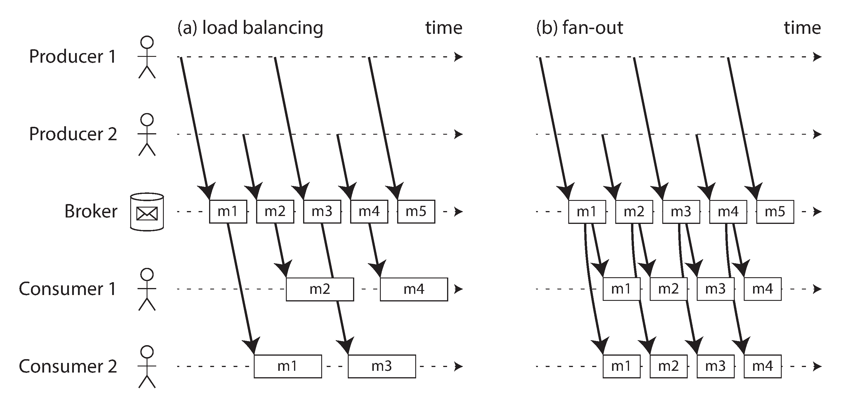
Figure 12-1 (a) Load balancing: sharing the work of consuming a topic among consumers; (b) fan-out: delivering each message to multiple consumers.

The two patterns can be combined, for example using Kafka’s consumer groups feature. When a consumer group subscribes to a topic, each message in the topic is sent to one of the consumers in the group (load-balancing across the consumers in the group). If two separate consumer groups subscribe to the same topic, each message is sent to one consumer in each group (providing fan-out across consumer groups).

Acknowledgments and redelivery

Consumers may crash at any time, so it could happen that a broker delivers a message to a consumer but the consumer never processes it, or only partially processes it before crashing. In order to ensure that the message is not lost, message brokers use acknowledgments: a client must explicitly tell the broker when it has finished processing a message so that the broker can remove it from the queue.

If the connection to a client is closed or times out without the broker receiving an acknowledgment, it assumes that the message was not processed, and therefore it delivers the message again to another consumer. (Note that it could happen that the message actually was fully processed, but the acknowledgment was lost in the network. Handling this case requires an atomic commit protocol, as discussed in “Exactly-once message processing”, unless the operation was idempotent or exactly-once semantics are not required.)

When combined with load balancing, this redelivery behavior has an interesting effect on the ordering of messages. In Figure 12-2, the consumers generally process messages in the order they were sent by producers. However, consumer 2 crashes while processing message m3, at the same time as consumer 1 is processing message m4. The unacknowledged message m3 is subsequently redelivered to consumer 1, with the result that consumer 1 processes messages in the order m4, m3, m5. Thus, m3 and m4 are not delivered in the same order as they were sent by producer 1.

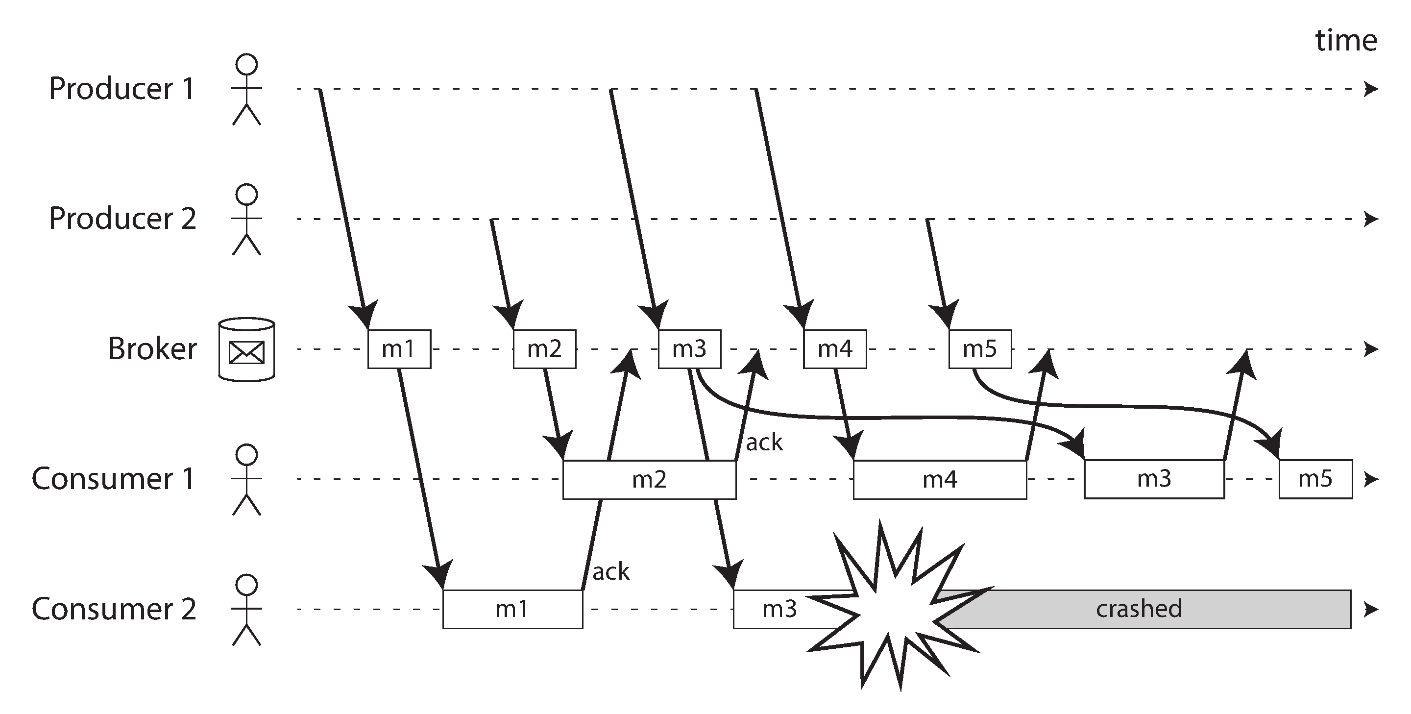
Figure 12-2 Consumer 2 crashes while processing m3, so it is redelivered to consumer 1 at a later time.

Even if the message broker otherwise tries to preserve the order of messages (as required by both the JMS and AMQP standards), the combination of load balancing with redelivery inevitably leads to messages being reordered. To avoid this issue, you can use a separate queue per consumer (i.e., not use the load balancing feature). Message reordering is not a problem if messages are completely independent of each other, but it can be important if there are causal dependencies between messages, as we shall see later in the chapter.

Redelivery can also result in wasted resources, resource starvation, or permanent blockages in a stream. A common scenario is a producer that improperly serializes a message; for example, by leaving out a required key in a JSON-encoded object. Any consumer that reads the message will expect the key, and fail if it’s missing. No acknowledgement is sent, so the broker will re-send the message, which will cause another consumer to fail. This loop repeats itself indefinitely. If the broker guarantees strong ordering, no further progress can be made. Brokers that allow message reordering can continue to make progress, but will waste resources on messages that will never be acknowledged.

Dead letter queues (DLQs) are used to handle this problem. Rather than keeping the message in the current queue and retrying forever, the message is moved to a different queue to unblock consumers ¹⁷, ¹⁸. Monitoring is usually set up on dead letter queues—any message in the queue is an error. Once a new message is detected, an operator can decide to permanently drop it, manually modify and re-produce the message, or fix consumer code to handle the message appropriately. DLQs are common in most queuing systems, but log-based messaging systems such as Apache Pulsar and stream processing systems such as Kafka Streams now support them as well ¹⁹.

Log-based Message Brokers

Sending a packet over a network or making a request to a network service is normally a transient operation that leaves no permanent trace. Although it is possible to record it permanently (using packet capture and logging), we normally don’t think of it that way. AMQP/JMS-style message brokers inherited this transient messaging mindset: even though they may write messages to disk, they quickly delete the messages again after they have been delivered to consumers.

Databases and filesystems take the opposite approach: everything that is written to a database or file is normally expected to be permanently recorded, at least until someone explicitly chooses to delete it again.

This difference in mindset has a big impact on how derived data is created. A key feature of batch processes, as discussed in Chapter 11, is that you can run them repeatedly, experimenting with the processing steps, without risk of damaging the input (since the input is read-only). This is not the case with AMQP/JMS-style messaging: receiving a message is destructive if the acknowledgment causes it to be deleted from the broker, so you cannot run the same consumer again and expect to get the same result.

If you add a new consumer to a messaging system, it typically only starts receiving messages sent after the time it was registered; any prior messages are already gone and cannot be recovered. Contrast this with files and databases, where you can add a new client at any time, and it can read data written arbitrarily far in the past (as long as it has not been explicitly overwritten or deleted by the application).

Why can we not have a hybrid, combining the durable storage approach of databases with the low-latency notification facilities of messaging? This is the idea behind log-based message brokers, which have become very popular in recent years.

Using logs for message storage

A log is simply an append-only sequence of records on disk. We previously discussed logs in the context of log-structured storage engines and write-ahead logs in Chapter 4, in the context of replication in Chapter 6, and as a form of consensus in Chapter 10.

The same structure can be used to implement a message broker: a producer sends a message by appending it to the end of the log, and a consumer receives messages by reading the log sequentially. If a consumer reaches the end of the log, it waits for a notification that a new message has been appended. The Unix tool tail -f, which watches a file for data being appended, essentially works like this.

In order to scale to higher throughput than a single disk can offer, the log can be sharded (in the sense of Chapter 7). Different shards can then be hosted on different machines, making each shard a separate log that can be read and written independently from other shards. A topic can then be defined as a group of shards that all carry messages of the same type. This approach is illustrated in Figure 12-3.

Within each shard, which Kafka calls a partition, the broker assigns a monotonically increasing sequence number, or offset, to every message (in Figure 12-3, the numbers in boxes are message offsets). Such a sequence number makes sense because a partition (shard) is append-only, so the messages within a partition are totally ordered. There is no ordering guarantee across different partitions.

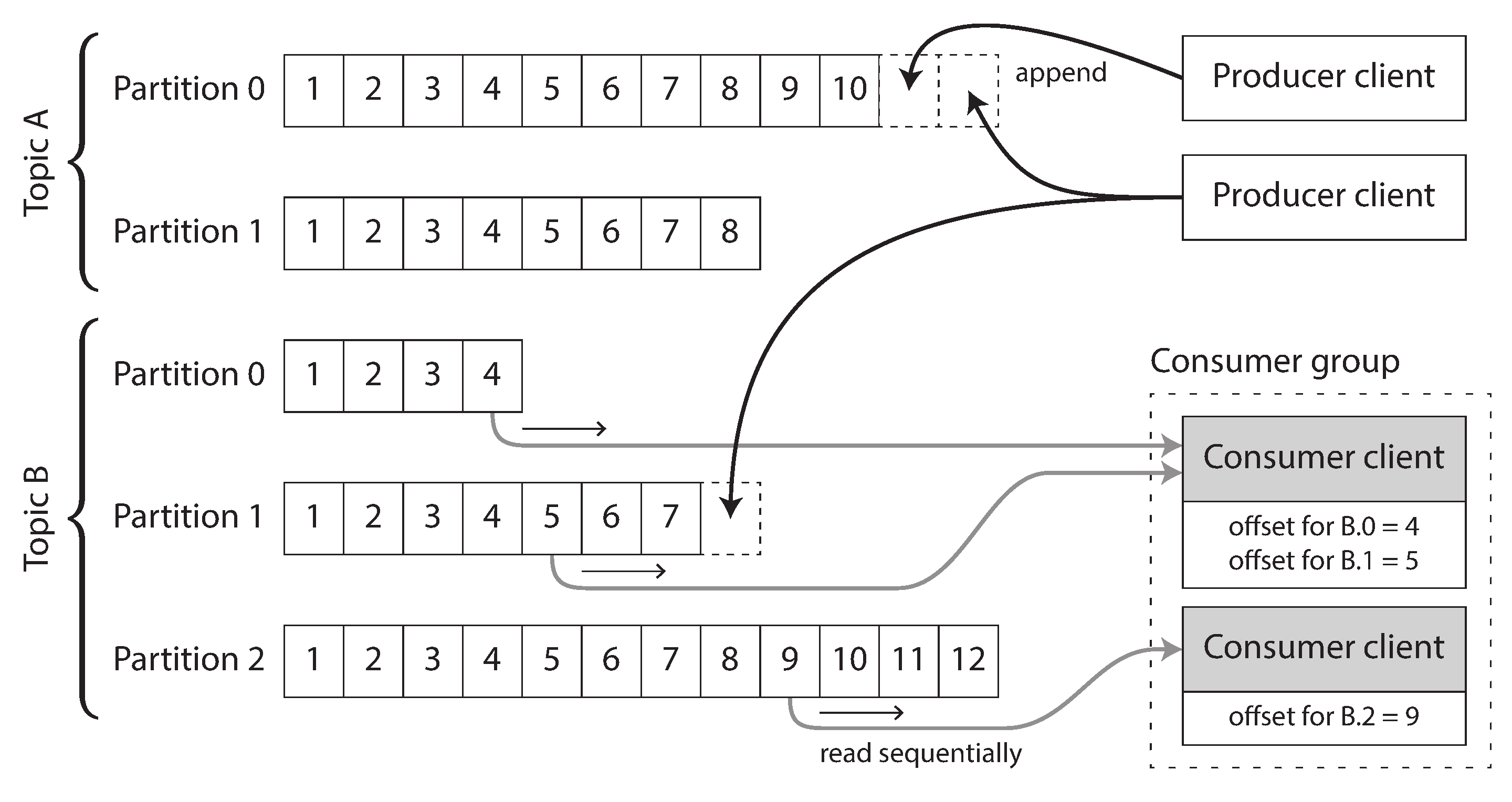
Figure 12-3 Producers send messages by appending them to a topic-partition file, and consumers read these files sequentially.

Apache Kafka ²⁰ and Amazon Kinesis Streams are log-based message brokers that work like this. Google Cloud Pub/Sub is architecturally similar but exposes a JMS-style API rather than a log abstraction ¹⁵. Even though these message brokers write all messages to disk, they are able to achieve throughput of millions of messages per second by sharding across multiple machines, and fault tolerance by replicating messages ²¹, ²².

Logs compared to traditional messaging

The log-based approach trivially supports fan-out messaging, because several consumers can independently read the log without affecting each other—reading a message does not delete it from the log. To achieve load balancing across a group of consumers, instead of assigning individual messages to consumer clients, the broker can assign entire shards to nodes in the consumer group.

Each client then consumes all the messages in the shards it has been assigned. Typically, when a consumer has been assigned a log shard, it reads the messages in the shard sequentially, in a straightforward single-threaded manner. This coarse-grained load balancing approach has some downsides:

The number of nodes sharing the work of consuming a topic can be at most the number of log shards in that topic, because messages within the same shard are delivered to the same node. (It’s possible to create a load balancing scheme in which two consumers share the work of processing a shard by having both read the full set of messages, but one of them only considers messages with even-numbered offsets while the other deals with the odd-numbered offsets. Alternatively, you could spread message processing over a thread pool, but that approach complicates consumer offset management. In general, single-threaded processing of a shard is preferable, and parallelism can be increased by using more shards.)
If a single message is slow to process, it holds up the processing of subsequent messages in that shard (a form of head-of-line blocking; see “Describing Performance”).

Thus, in situations where messages may be expensive to process and you want to parallelize processing on a message-by-message basis, and where message ordering is not so important, the JMS/AMQP style of message broker is preferable. On the other hand, in situations with high message throughput, where each message is fast to process and where message ordering is important, the log-based approach works very well ²³, ²⁴. However, the distinction between the two architectures is being blurred as log-based messaging systems such as Kafka now support JMS/AMQP style consumer groups, which allow multiple consumers to receive messages from the same partition ²⁵, ²⁶.

Since sharded logs typically preserve message ordering only within a single shard, all messages that need to be ordered consistently need to be routed to the same shard. For example, an application may require that the events relating to one particular user appear in a fixed order. This can be achieved by choosing the shard for an event based on the user ID of that event (in other words, making the user ID the partition key).

Consumer offsets

Consuming a shard sequentially makes it easy to tell which messages have been processed: all messages with an offset less than a consumer’s current offset have already been processed, and all messages with a greater offset have not yet been seen. Thus, the broker does not need to track acknowledgments for every single message—it only needs to periodically record the consumer offsets. The reduced bookkeeping overhead and the opportunities for batching and pipelining in this approach help increase the throughput of log-based systems. If a consumer fails, however, it will resume from the last recorded offset rather than the more recent last offset it saw. This can causes the consumer to see some messages twice.

This offset is in fact very similar to the log sequence number that is commonly found in single-leader database replication, and which we discussed in “Setting Up New Followers”. In database replication, the log sequence number allows a follower to reconnect to a leader after it has become disconnected, and resume replication without skipping any writes. Exactly the same principle is used here: the message broker behaves like a leader database, and the consumer like a follower.

If a consumer node fails, another node in the consumer group is assigned the failed consumer’s shards, and it starts consuming messages at the last recorded offset. If the consumer had processed subsequent messages but not yet recorded their offset, those messages will be processed a second time upon restart. We will discuss ways of dealing with this issue later in the chapter.

Disk space usage

If you only ever append to the log, you will eventually run out of disk space. To reclaim disk space, the log is actually divided into segments, and from time to time old segments are deleted or moved to archive storage. (We’ll discuss a more sophisticated way of freeing disk space in “Log compaction”.)

This means that if a slow consumer cannot keep up with the rate of messages, and it falls so far behind that its consumer offset points to a deleted segment, it will miss some of the messages. Effectively, the log implements a bounded-size buffer that discards old messages when it gets full, also known as a circular buffer or ring buffer. However, since that buffer is on disk, it can be quite large.

Let’s do a back-of-the-envelope calculation. At the time of writing, a typical large hard drive has a capacity of 20 TB and a sequential write throughput of 250 MB/s. If you are writing messages at the fastest possible rate, it takes about 22 hours until the drive is full and you need to start deleting the oldest messages. That means a disk-based log can always buffer at least 22 hours worth of messages, even if you have many disks with many machines (having more disks increases both the available space and the total write bandwidth). In practice, deployments rarely use the full write bandwidth of the disk, so the log can typically keep a buffer of several days’ or even weeks’ worth of messages.

Many log-based message brokers now store messages in object storage to increase their storage capacity, similarly to databases as we saw in “Databases Backed by Object Storage”. Message brokers such as Apache Kafka and Redpanda serve older messages from object storage as part of their tiered storage. Others, such as WarpStream, Confluent Freight, and Bufstream store all of their data in the object store. In addition to cost-efficiency, this architecture also makes data integration easier: messages in object storage are stored as Iceberg tables, which enable batch and data warehouse job execution directly on the data without having to copy it into another system.

When consumers cannot keep up with producers

At the beginning of “Messaging Systems” we discussed three choices of what to do if a consumer cannot keep up with the rate at which producers are sending messages: dropping messages, buffering, or applying backpressure. In this taxonomy, the log-based approach is a form of buffering with a large but fixed-size buffer (limited by the available disk space).

If a consumer falls so far behind that the messages it requires are older than what is retained on disk, it will not be able to read those messages—so the broker effectively drops old messages that go back further than the size of the buffer can accommodate. You can monitor how far a consumer is behind the head of the log, and raise an alert if it falls behind significantly. As the buffer is large, there is enough time for a human operator to fix the slow consumer and allow it to catch up before it starts missing messages.

Even if a consumer does fall too far behind and starts missing messages, only that consumer is affected; it does not disrupt the service for other consumers. This fact is a big operational advantage: you can experimentally consume a production log for development, testing, or debugging purposes, without having to worry much about disrupting production services. When a consumer is shut down or crashes, it stops consuming resources—the only thing that remains is its consumer offset.

This behavior also contrasts with traditional message brokers, where you need to be careful to delete any queues whose consumers have been shut down—otherwise they continue unnecessarily accumulating messages and taking away memory from consumers that are still active.

Replaying old messages

We noted previously that with AMQP- and JMS-style message brokers, processing and acknowledging messages is a destructive operation, since it causes the messages to be deleted on the broker. On the other hand, in a log-based message broker, consuming messages is more like reading from a file: it is a read-only operation that does not change the log.

The only side effect of processing, besides any output of the consumer, is that the consumer offset moves forward. But the offset is under the consumer’s control, so it can easily be manipulated if necessary: for example, you can start a copy of a consumer with yesterday’s offsets and write the output to a different location, in order to reprocess the last day’s worth of messages. You can repeat this any number of times, varying the processing code.

This aspect makes log-based messaging more like the batch processes of the last chapter, where derived data is clearly separated from input data through a repeatable transformation process. It allows more experimentation and easier recovery from errors and bugs, making it a good tool for integrating dataflows within an organization ²⁷.

Databases and Streams

We have drawn some comparisons between message brokers and databases. Even though they have traditionally been considered separate categories of tools, we saw that log-based message brokers have been successful in taking ideas from databases and applying them to messaging. We can also go in reverse: take ideas from messaging and streams, and apply them to databases.

One approach is to use an event stream as the system of record for storing data (see “Systems of Record and Derived Data”). This is what happens in event sourcing, which we discussed in “Event Sourcing and CQRS”: instead of storing data in a data model that is mutated by updating and deleting, you can model every state change as an immutable event, and write it to an append-only log. Any read-optimized materialized views are derived from these events. Log-based message brokers (configured to never delete old events) are well suited for event sourcing since they use append-only storage, and they can notify consumers about new events with low latency.

But you don’t have to go as far as adopting event sourcing; even with mutable data models, event streams are useful for databases. In fact, every write to a database is an event that can be captured, stored, and processed. The connection between databases and streams runs deeper than just the physical storage of logs on disk—it is quite fundamental.

For example, a replication log (see “Implementation of Replication Logs”) is a stream of database write events, produced by the leader as it processes transactions. The followers apply that stream of writes to their own copy of the database and thus end up with an accurate copy of the same data. The events in the replication log describe the data changes that occurred.

We also came across the state machine replication principle in “Using shared logs”, which states: if every event represents a write to the database, and every replica processes the same events in the same order, then the replicas will all end up in the same final state. (Processing an event is assumed to be a deterministic operation.) It’s just another case of event streams!

In this section we will first look at a problem that arises in heterogeneous data systems, and then explore how we can solve it by bringing ideas from event streams to databases.

Keeping Systems in Sync

As we have seen throughout this book, there is no single system that can satisfy all data storage, querying, and processing needs. In practice, most nontrivial applications need to combine several different technologies in order to satisfy their requirements: for example, using an OLTP database to serve user requests, a cache to speed up common requests, a full-text index to handle search queries, and a data warehouse for analytics. Each of these has its own copy of the data, stored in its own representation that is optimized for its own purposes.

As the same or related data appears in several different places, they need to be kept in sync with one another: if an item is updated in the database, it also needs to be updated in the cache, search indexes, and data warehouse. With data warehouses this synchronization is usually performed by ETL processes (see “Data Warehousing”), often by taking a full copy of a database, transforming it, and bulk-loading it into the data warehouse—in other words, a batch process. Similarly, we saw in “Batch Use Cases” how search indexes, recommendation systems, and other derived data systems might be created using batch processes.

If periodic full database dumps are too slow, an alternative that is sometimes used is dual writes, in which the application code explicitly writes to each of the systems when data changes: for example, first writing to the database, then updating the search index, then invalidating the cache entries (or even performing those writes concurrently).

However, dual writes have some serious problems, one of which is a race condition illustrated in Figure 12-4. In this example, two clients concurrently want to update an item X: client 1 wants to set the value to A, and client 2 wants to set it to B. Both clients first write the new value to the database, then write it to the search index. Due to unlucky timing, the requests are interleaved: the database first sees the write from client 1 setting the value to A, then the write from client 2 setting the value to B, so the final value in the database is B. The search index first sees the write from client 2, then client 1, so the final value in the search index is A. The two systems are now permanently inconsistent with each other, even though no error occurred.

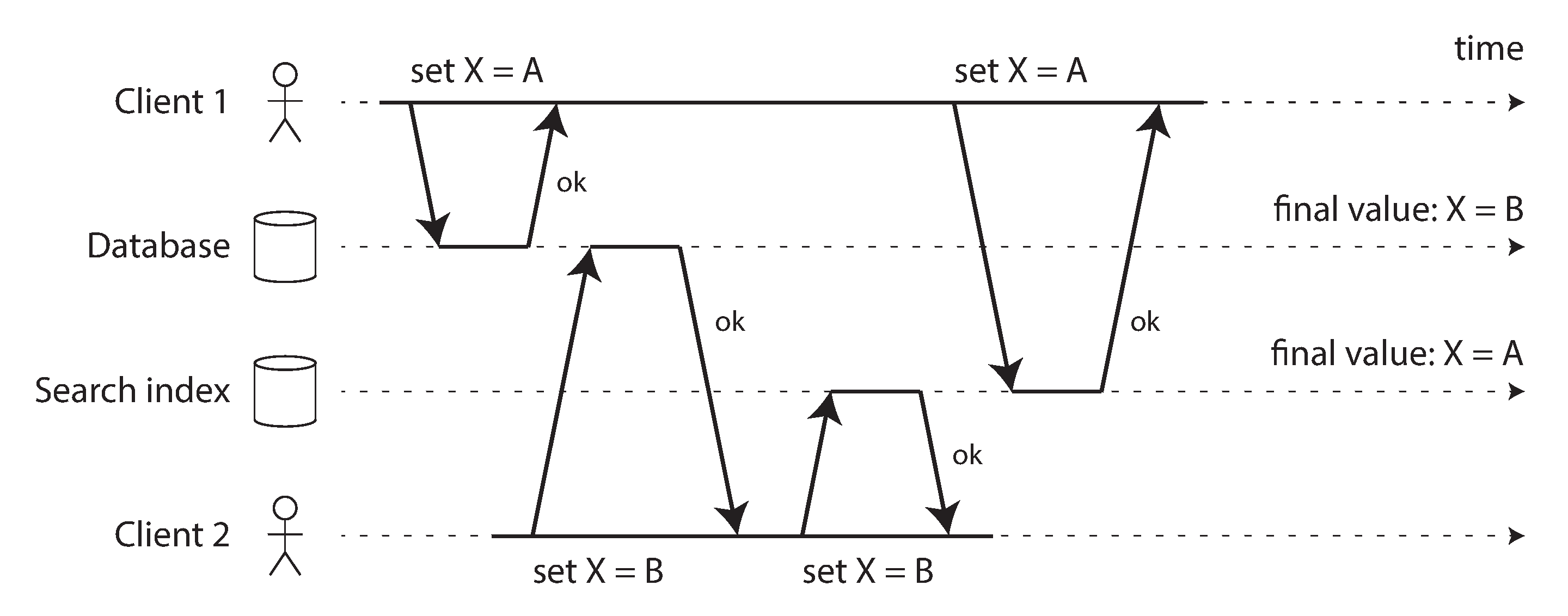
Figure 12-4 In the database, X is first set to A and then to B, while at the search index the writes arrive in the opposite order.

Unless you have some additional concurrency detection mechanism, such as the version vectors we discussed in “Detecting Concurrent Writes”, you will not even notice that concurrent writes occurred—one value will simply silently overwrite another value.

Another problem with dual writes is that one of the writes may fail while the other succeeds. This is a fault-tolerance problem rather than a concurrency problem, but it also has the effect of the two systems becoming inconsistent with each other. Ensuring that they either both succeed or both fail is a case of the atomic commit problem, which is expensive to solve (see “Two-Phase Commit (2PC)”).

If you only have one replicated database with a single leader, then that leader determines the order of writes, so the state machine replication approach works among replicas of the database. However, in Figure 12-4 there isn’t a single leader: the database may have a leader and the search index may have a leader, but neither follows the other, and so conflicts can occur (see “Multi-Leader Replication”).

The situation would be better if there really was only one leader—for example, the database—and if we could make the search index a follower of the database. But is this possible in practice?

Change Data Capture

The problem with most databases’ replication logs is that they have long been considered to be an internal implementation detail of the database, not a public API. Clients are supposed to query the database through its data model and query language, not parse the replication logs and try to extract data from them.

For decades, many databases simply did not have a documented way of getting the log of changes written to them. For this reason it was difficult to take all the changes made in a database and replicate them to a different storage technology such as a search index, cache, or data warehouse.

More recently, there has been growing interest in change data capture (CDC), which is the process of observing all data changes written to a database and extracting them in a form in which they can be replicated to other systems ²⁸. CDC is especially interesting if changes are made available as a stream, immediately as they are written.

For example, you can capture the changes in a database and continually apply the same changes to a search index. If the log of changes is applied in the same order, you can expect the data in the search index to match the data in the database. The search index and any other derived data systems are just consumers of the change stream.

Figure 12-5 shows how the concurrency problem of Figure 12-4 is solved with CDC. Even though the two requests to set X to A and B respectively arrive concurrently at the database, the database decides on some order in which to execute them, and writes them to its replication log in that order. The search index picks them up and applies them in the same order. If you need the data in another system, such as a data warehouse, you can simply add it as another consumer of the CDC event stream.

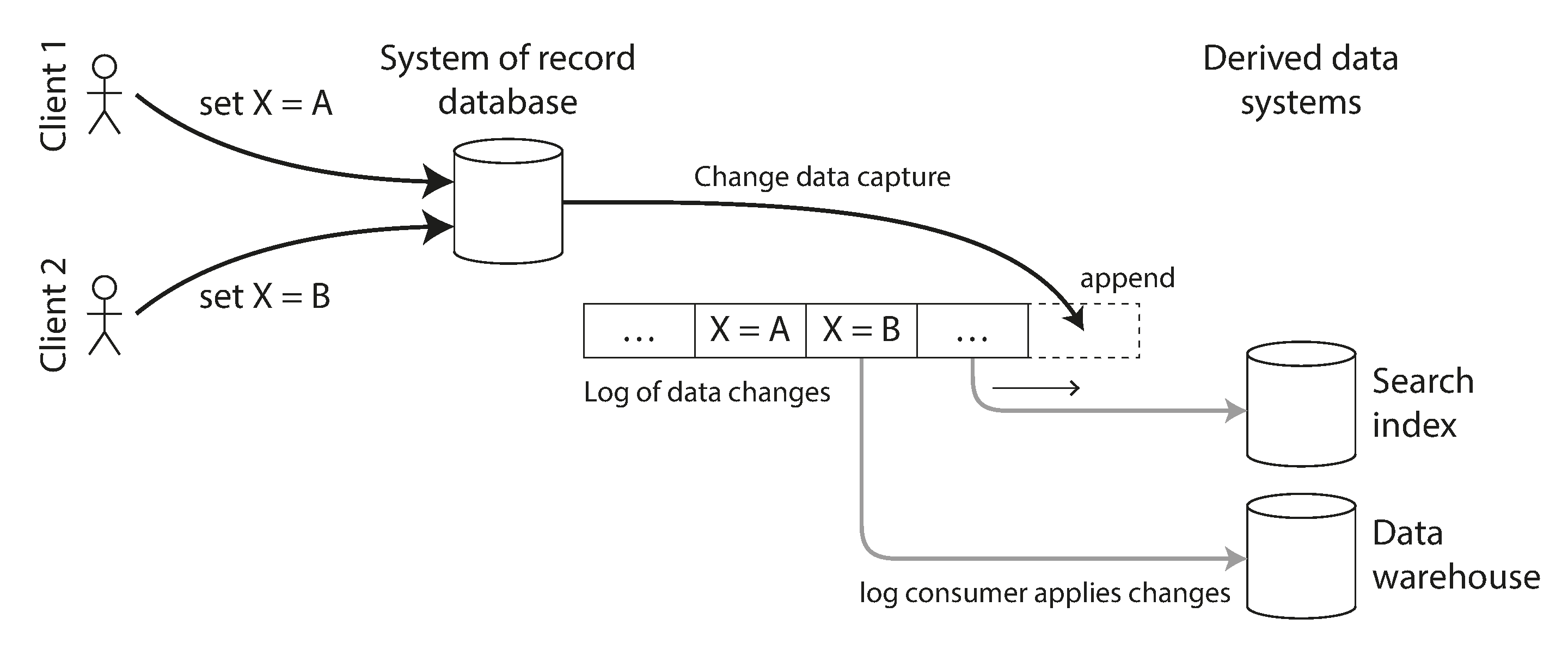
Figure 12-5 Taking data in the order it was written to one database, and applying the changes to other systems in the same order.

Implementing change data capture

We can call the log consumers derived data systems, as discussed in “Systems of Record and Derived Data”: the data stored in the search index and the data warehouse is just another view onto the data in the system of record. Change data capture is a mechanism for ensuring that all changes made to the system of record are also reflected in the derived data systems so that the derived systems have an accurate copy of the data.

Essentially, change data capture makes one database the leader (the one from which the changes are captured), and turns the others into followers. A log-based message broker is well suited for transporting the change events from the source database to the derived systems, since it preserves the ordering of messages (avoiding the reordering issue of Figure 12-2).

Logical replication logs can be used to implement change data capture (see “Logical (row-based) log replication”), although it comes with challenges, such as handling schema changes and properly modeling updates. The Debezium open source project addresses these challenges. The project contains source connectors for MySQL, PostgreSQL, Oracle, SQL Server, Db2, Cassandra, and many other databases. These connectors attach to database replication logs and surface the changes in a standard event schema. Messages can then be transformed and written to downstream databases. The Kafka Connect framework offers further CDC connectors for various databases, as well. Maxwell does something similar for MySQL by parsing the binlog ²⁹, GoldenGate provides similar facilities for Oracle, and pgcapture does the same for PostgreSQL.

Like message brokers, change data capture is usually asynchronous: the system of record database does not wait for the change to be applied to consumers before committing it. This design has the operational advantage that adding a slow consumer does not affect the system of record too much, but it has the downside that all the issues of replication lag apply (see “Problems with Replication Lag”).

Initial snapshot

If you have the log of all changes that were ever made to a database, you can reconstruct the entire state of the database by replaying the log. However, in many cases, keeping all changes forever would require too much disk space, and replaying it would take too long, so the log needs to be truncated.

Building a new full-text index, for example, requires a full copy of the entire database—it is not sufficient to only apply a log of recent changes, since it would be missing items that were not recently updated. Thus, if you don’t have the entire log history, you need to start with a consistent snapshot, as previously discussed in “Setting Up New Followers”.

The snapshot of the database must correspond to a known position or offset in the change log, so that you know at which point to start applying changes after the snapshot has been processed. Some CDC tools integrate this snapshot facility, while others leave it as a manual operation. Debezium uses Netflix’s DBLog watermarking algorithm to provide incremental snapshots ³⁰, ³¹.

Log compaction

If you can only keep a limited amount of log history, you need to go through the snapshot process every time you want to add a new derived data system. However, log compaction provides a good alternative.

We discussed log compaction previously in “Log-Structured Storage”, in the context of log-structured storage engines (see Figure 4-3 for an example). The principle is simple: the storage engine periodically looks for log records with the same key, throws away any duplicates, and keeps only the most recent update for each key. This might make log segments much smaller, so segments may also be merged as part of the compaction process, as shown in Figure 12-6. This process runs in the background.

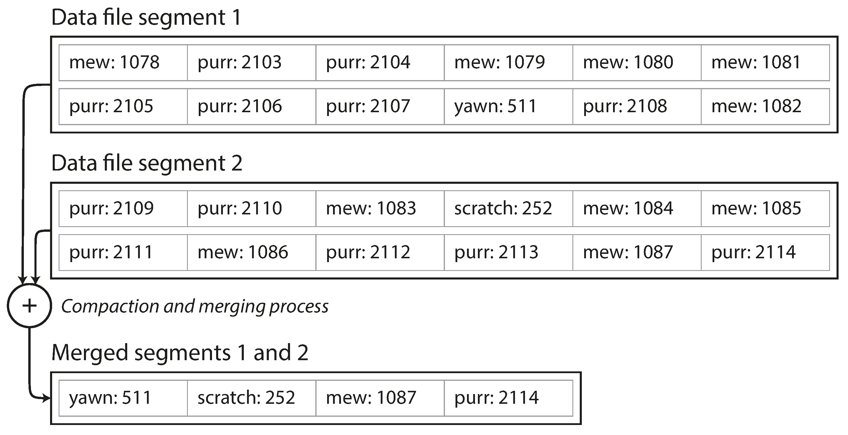
Figure 12-6 A log of key-value pairs, where the key is the ID of a cat video (mew, purr, scratch, or yawn), and the value is the number of times it has been played. Log compaction retains only the most recent value for each key.

In a log-structured storage engine, an update with a special null value (a tombstone) indicates that a key was deleted, and causes it to be removed during log compaction. But as long as a key is not overwritten or deleted, it stays in the log forever. The disk space required for such a compacted log depends only on the current contents of the database, not the number of writes that have ever occurred in the database. If the same key is frequently overwritten, previous values will eventually be garbage-collected, and only the latest value will be retained.

The same idea works in the context of log-based message brokers and change data capture. If the CDC system is set up such that every change has a primary key, and every update for a key replaces the previous value for that key, then it’s sufficient to keep just the most recent write for a particular key.

Now, whenever you want to rebuild a derived data system such as a search index, you can start a new consumer from offset 0 of the log-compacted topic, and sequentially scan over all messages in the log. The log is guaranteed to contain the most recent value for every key in the database (and maybe some older values)—in other words, you can use it to obtain a full copy of the database contents without having to take another snapshot of the CDC source database.

This log compaction feature is supported by Apache Kafka. As we shall see later in this chapter, it allows the message broker to be used for durable storage, not just for transient messaging.

API support for change streams

Most popular databases now expose change streams as a first-class interface, rather than the retrofitted and reverse-engineered CDC efforts of the past. Relational databases such as MySQL and PostgreSQL typically send changes through the same replication log they use for their own replicas. Most cloud vendors offer CDC solutions for their products as well: for example, Datastream offers streaming data access for Google Cloud’s relational databases and data warehouses.

Even evenutally consistent, quorum-based databases such as Cassandra now support change data capture. As we saw in “Linearizability and quorums”, clients must persist writes to a majority of nodes before they’re considered visible. CDC support for quorum writes is challenging because there’s no single source of truth to subscribe to. Whether the data is visible or not depends on each reader’s consistency preferences. Cassandra sidesteps this issue by exposing raw log segments for each node rather than providing a single stream of mutations. Systems that wish to consume the data must read the raw log segments for each node and decide how best to merge them into a single stream (much like a quorum reader does) ³².

Kafka Connect ³³ integrates change data capture tools for a wide range of database systems with Kafka. Once the stream of change events is in Kafka, it can be used to update derived data systems such as search indexes, and also feed into stream processing systems as discussed later in this chapter.

Change data capture versus event sourcing

Let’s compare change data capture to event sourcing. Similarly to change data capture, event sourcing involves storing all changes to the application state as a log of change events. The biggest difference is that event sourcing applies the idea at a different level of abstraction:

In change data capture, the application uses the database in a mutable way, updating and deleting records at will. The log of changes is extracted from the database at a low level (e.g., by parsing the replication log), which ensures that the order of writes extracted from the database matches the order in which they were actually written, avoiding the race condition in Figure 12-4.
In event sourcing, the application logic is explicitly built on the basis of immutable events that are written to an event log. In this case, the event store is append-only, and updates or deletes of events are discouraged or prohibited. Events are designed to reflect things that happened at the application level, rather than low-level state changes.

Which one is better depends on your situation. Adopting event sourcing is a big change for an application that is not already doing it; it has a number of pros and cons, which we discussed in “Event Sourcing and CQRS”. In contrast, CDC can be added to an existing database with minimal changes—the application writing to the database might not even know that CDC is occurring.

CHANGE DATA CAPTURE AND DATABASE SCHEMAS

Though change data capture appears easier to adopt than event sourcing, it comes with its own set of challenges.

In a microservices architecture, a database is typically only accessed from one service. Other services interact with it through that service’s public API, but they don’t normally access the database directly. This makes the database an internal implementation detail of the service, allowing the developers to change its database schema without affecting the public API.

However, CDC systems typically use the upstream database’s schema when replicating its data, which turns these schemas into public APIs that must be managed much like the public API of the service. A developer who removes a table column in their database table will break downstream consumers that depend on this field. Such challenges have always existed with data pipelines, but they typically only impacted data warehouse ETL. Since CDC is often implemented as a data stream, other production services might be consumers. Breaking such consumers can cause a customer-facing outage ³⁴. Data contracts are often used to prevent these breakages.

A common way to decouple internal from external schemas is to use the outbox pattern. Outboxes are tables with their own schemas, which are exposed to the CDC system rather than the internal domain model in the database ³⁵, ³⁶. Developers can then modify their internal schemas as they see fit while leaving their outbox tables untouched. This might look like a dual write—it is. However, outboxes avoid the challenges we discussed in “Keeping Systems in Sync” by keeping both writes in the same system (the database). This design allows both writes to appear in a single transaction.

Outboxes present a few tradeoffs, though. Developers must still maintain the transformation between their internal and outbox schemas, which can be challenging. An outbox also increases the amount of data that the database has to write to its underlying storage, which might trigger performance problems.

Like with change data capture, replaying the event log allows you to reconstruct the current state of the system. However, log compaction needs to be handled differently:

A CDC event for the update of a record typically contains the entire new version of the record, so the current value for a primary key is entirely determined by the most recent event for that primary key, and log compaction can discard previous events for the same key.
On the other hand, with event sourcing, events are modeled at a higher level: an event typically expresses the intent of a user action, not the mechanics of the state update that occurred as a result of the action. In this case, later events typically do not override prior events, and so you need the full history of events to reconstruct the final state. Log compaction is not possible in the same way.

Applications that use event sourcing typically have some mechanism for storing snapshots of the current state that is derived from the log of events, so they don’t need to repeatedly reprocess the full log. However, this is only a performance optimization to speed up reads and recovery from crashes; the intention is that the system is able to store all raw events forever and reprocess the full event log whenever required. We discuss this assumption in “Limitations of immutability”.

State, Streams, and Immutability

We saw in Chapter 11 that batch processing benefits from the immutability of its input files, so you can run experimental processing jobs on existing input files without fear of damaging them. This principle of immutability is also what makes event sourcing and change data capture so powerful.

We normally think of databases as storing the current state of the application—this representation is optimized for reads, and it is usually the most convenient for serving queries. The nature of state is that it changes, so databases support updating and deleting data as well as inserting it. How does this fit with immutability?

Whenever you have state that changes, that state is the result of the events that mutated it over time. For example, your list of currently available seats is the result of the reservations you have processed, the current account balance is the result of the credits and debits on the account, and the response time graph for your web server is an aggregation of the individual response times of all web requests that have occurred.

No matter how the state changes, there was always a sequence of events that caused those changes. Even as things are done and undone, the fact remains true that those events occurred. The key idea is that mutable state and an append-only log of immutable events do not contradict each other: they are two sides of the same coin. The log of all changes, the changelog, represents the evolution of state over time.

If you are mathematically inclined, you might say that the application state is what you get when you integrate an event stream over time, and a change stream is what you get when you differentiate the state by time, as shown in Figure 12-7 ³⁷, ³⁸. The analogy has limitations (for example, the second derivative of state does not seem to be meaningful), but it’s a useful starting point for thinking about data.

Figure 12-7 The relationship between the current application state and an event stream.

If you store the changelog durably, that simply has the effect of making the state reproducible. If you consider the log of events to be your system of record, and any mutable state as being derived from it, it becomes easier to reason about the flow of data through a system. As Jim Gray and Andreas Reuter put it in 1992 ³⁹:

[T]here is no fundamental need to keep a database at all; the log contains all the information there is. The only reason for storing the database (i.e., the current end-of-the-log) is performance of retrieval operations.

Log compaction is one way of bridging the distinction between log and database state: it retains only the latest version of each record, and discards overwritten versions.

Advantages of immutable events

Immutability in databases is an old idea. For example, accountants have been using immutability for centuries in financial bookkeeping. When a transaction occurs, it is recorded in an append-only ledger, which is essentially a log of events describing money, goods, or services that have changed hands. The accounts, such as profit and loss or the balance sheet, are derived from the transactions in the ledger by adding them up ⁴⁰.

If a mistake is made, accountants don’t erase or change the incorrect transaction in the ledger—instead, they add another transaction that compensates for the mistake, for example refunding an incorrect charge. The incorrect transaction still remains in the ledger forever, because it might be important for auditing reasons. If incorrect figures, derived from the incorrect ledger, have already been published, then the figures for the next accounting period include a correction. This process is entirely normal in accounting ⁴¹.

Although such auditability is particularly important in financial systems, it is also beneficial for many other systems that are not subject to such strict regulation. If you accidentally deploy buggy code that writes bad data to a database, recovery is much harder if the code is able to destructively overwrite data. With an append-only log of immutable events, it is much easier to diagnose what happened and recover from the problem. Similarly, customer service can use an audit log to diagnose customer requests and complaints.

Immutable events also capture more information than just the current state. For example, on a shopping website, a customer may add an item to their cart and then remove it again. Although the second event cancels out the first event from the point of view of order fulfillment, it may be useful to know for analytics purposes that the customer was considering a particular item but then decided against it. Perhaps they will choose to buy it in the future, or perhaps they found a substitute. This information is recorded in an event log, but would be lost in a database that deletes items when they are removed from the cart.

Deriving several views from the same event log

Moreover, by separating mutable state from the immutable event log, you can derive several different read-oriented representations from the same log of events. This works just like having multiple consumers of a stream (Figure 12-5): for example, the analytic database Druid ingests directly from Kafka using this approach, and Kafka Connect sinks can export data from Kafka to various different databases and indexes ³³.

Having an explicit translation step from an event log to a database makes it easier to evolve your application over time: if you want to introduce a new feature that presents your existing data in some new way, you can use the event log to build a separate read-optimized view for the new feature, and run it alongside the existing systems without having to modify them. Running old and new systems side by side is often easier than performing a complicated schema migration in an existing system. Once readers have switched to the new system and the old system is no longer needed, you can simply shut it down and reclaim its resources ⁴², ⁴³.

This idea of writing data in one write-optimized form, and then translating it into different read-optimized representations as needed, is the command query responsibility segregation (CQRS) pattern that we already encountered in “Event Sourcing and CQRS”. It doesn’t necessarily require event sourcing: you can just as well build multiple materialized views from a stream of CDC events ⁴⁴.

The traditional approach to database and schema design is based on the fallacy that data must be written in the same form as it will be queried. Debates about normalization and denormalization (see “Normalization, Denormalization, and Joins”) become largely irrelevant if you can translate data from a write-optimized event log to read-optimized application state: it is entirely reasonable to denormalize data in the read-optimized views, as the translation process gives you a mechanism for keeping it consistent with the event log.

In “Case Study: Social Network Home Timelines” we discussed a social network’s home timelines, a cache of recent posts by the people a particular user is following (like a mailbox). This is another example of read-optimized state: home timelines are highly denormalized, since your posts are duplicated in all of the timelines of the people following you. However, the fan-out service keeps this duplicated state in sync with new posts and new following relationships, which keeps the duplication manageable.

Concurrency control

The biggest downside of CQRS is that the consumers of the event log are usually asynchronous, so there is a possibility that a user may make a write to the log, then read from a derived view and find that their write has not yet been reflected in the view. We discussed this problem and potential solutions previously in “Reading Your Own Writes”.

One solution would be to perform the updates of the read view synchronously with appending the event to the log. This either requires a distributed transaction across the event log and the derived view, or some way of waiting until an event has been reflected in the view. Both approaches are usually impractical, so views are normally updated asynchronously.

On the other hand, deriving the current state from an event log also simplifies some aspects of concurrency control. Much of the need for multi-object transactions (see “Single-Object and Multi-Object Operations”) stems from a single user action requiring data to be changed in several different places. With event sourcing, you can design an event such that it is a self-contained description of a user action. The user action then requires only a single write in one place—namely appending the event to the log—which is easy to make atomic.

If the event log and the application state are sharded in the same way (for example, processing an event for a customer in shard 3 only requires updating shard 3 of the application state), then a straightforward single-threaded log consumer needs no concurrency control for writes—by construction, it only processes a single event at a time (see also “Actual Serial Execution”). The log removes the nondeterminism of concurrency by defining a serial order of events in a shard ²⁷. If an event touches multiple state shards, a bit more work is required, which we will discuss in Chapter 13.

Many systems that don’t use an event-sourced model nevertheless rely on immutability for concurrency control: various databases internally use immutable data structures or multi-version data to support point-in-time snapshots (see “Indexes and snapshot isolation”). Version control systems such as Git, Mercurial, and Fossil also rely on immutable data to preserve version history of files.

Limitations of immutability

To what extent is it feasible to keep an immutable history of all changes forever? The answer depends on the amount of churn in the dataset. Some workloads mostly add data and rarely update or delete; they are easy to make immutable. Other workloads have a high rate of updates and deletes on a comparatively small dataset; in these cases, the immutable history may grow prohibitively large, fragmentation may become an issue, and the performance of compaction and garbage collection becomes crucial for operational robustness ⁴⁵, ⁴⁶.

Besides the performance reasons, there may also be circumstances in which you need data to be deleted for administrative or legal reasons, in spite of all immutability. For example, privacy regulations such as the European General Data Protection Regulation (GDPR) require that a user’s personal information be deleted and erroneous information be removed on demand, or an accidental leak of sensitive information may need to be contained.

In these circumstances, it’s not sufficient to just append another event to the log to indicate that the prior data should be considered deleted—you actually want to rewrite history and pretend that the data was never written in the first place. For example, Datomic calls this feature excision ⁴⁷, and the Fossil version control system has a similar concept called shunning ⁴⁸.

Truly deleting data is surprisingly hard ⁴⁹, since copies can live in many places: for example, storage engines, filesystems, and SSDs often write to a new location rather than overwriting in place ⁴¹, and backups are often deliberately immutable to prevent accidental deletion or corruption.

One way of enabling deletion of immutable data is crypto-shredding ⁵⁰: data that you may want to delete in the future is stored encrypted, and when you want to get rid of it, you forget the encryption key. The encrypted data is then still there, but nobody can use it. In some sense this only moves the problem around: the actual data is now immutable, but your key storage is mutable.

Moreover, you have to decide up front which data is going to be encrypted with the same key, and when you are going to use different keys—an important decision, since you can later crypto-shred either all or none of the data encrypted with a particular key, but not some of it. Storing a separate key for every single data item would get too unwieldy, as the key storage would get as big as the primary data storage. More sophisticated schemes such as puncturable encryption ⁵¹ make it possible to selectively revoke a key’s decryption abilities, but they are not widely used.

Overall, deletion is more a matter of “making it harder to retrieve the data” than actually “making it impossible to retrieve the data.” Nevertheless, you sometimes have to try, as we shall see in “Legislation and Self-Regulation”.

Processing Streams

So far in this chapter we have talked about where streams come from (user activity events, sensors, and writes to databases), and we have talked about how streams are transported (through direct messaging, via message brokers, and in event logs).

What remains is to discuss what you can do with the stream once you have it—namely, you can process it. Broadly, there are three options:

You can take the data in the events and write it to a database, cache, search index, or similar storage system, from where it can then be queried by other clients. As shown in Figure 12-5, this is a good way of keeping a database in sync with changes happening in other parts of the system—especially if the stream consumer is the only client writing to the database. Writing to a storage system is the streaming equivalent of what we discussed in “Batch Use Cases”.
You can push the events to users in some way, for example by sending email alerts or push notifications, or by streaming the events to a real-time dashboard where they are visualized. In this case, a human is the ultimate consumer of the stream.
You can process one or more input streams to produce one or more output streams. Streams may go through a pipeline consisting of several such processing stages before they eventually end up at an output (option 1 or 2).

In the rest of this chapter, we will discuss option 3: processing streams to produce other, derived streams. A piece of code that processes streams like this is known as an operator or a job. It is closely related to the Unix processes and MapReduce jobs we discussed in Chapter 11, and the pattern of dataflow is similar: a stream processor consumes input streams in a read-only fashion and writes its output to a different location in an append-only fashion.

The patterns for sharding and parallelization in stream processors are also very similar to those in MapReduce and the dataflow engines we saw in Chapter 11, so we won’t repeat those topics here. Basic mapping operations such as transforming and filtering records also work the same.

The one crucial difference from batch jobs is that a stream never ends. This difference has many implications: as discussed at the start of this chapter, sorting does not make sense with an unbounded dataset, and so sort-merge joins (see “JOIN and GROUP BY”) cannot be used. Fault-tolerance mechanisms must also change: with a batch job that has been running for a few minutes, a failed task can simply be restarted from the beginning, but with a stream job that has been running for several years, restarting from the beginning after a crash may not be a viable option.

Uses of Stream Processing

Stream processing has long been used for monitoring purposes, where an organization wants to be alerted if certain things happen. For example:

Fraud detection systems need to determine if the usage patterns of a credit card have unexpectedly changed, and block the card if it is likely to have been stolen.
Trading systems need to examine price changes in a financial market and execute trades according to specified rules.
Manufacturing systems need to monitor the status of machines in a factory, and quickly identify the problem if there is a malfunction.
Military and intelligence systems need to track the activities of a potential aggressor, and raise the alarm if there are signs of an attack.

These kinds of applications require quite sophisticated pattern matching and correlations. However, other uses of stream processing have also emerged over time. In this section we will briefly compare and contrast some of these applications.

Complex event processing

Complex event processing (CEP) is an approach developed in the 1990s for analyzing event streams, especially geared toward the kind of application that requires searching for certain event patterns ⁵². Similarly to the way that a regular expression allows you to search for certain patterns of characters in a string, CEP allows you to specify rules to search for certain patterns of events in a stream.

CEP systems often use a high-level declarative query language like SQL, or a graphical user interface, to describe the patterns of events that should be detected. These queries are submitted to a processing engine that consumes the input streams and internally maintains a state machine that performs the required matching. When a match is found, the engine emits a complex event (hence the name) with the details of the event pattern that was detected ⁵³.

In these systems, the relationship between queries and data is reversed compared to normal databases. Usually, a database stores data persistently and treats queries as transient: when a query comes in, the database searches for data matching the query, and then forgets about the query when it has finished. CEP engines reverse these roles: queries are stored long-term; as each event arrives, the engine checks whether it has now seen an event pattern that matches any of its standing queries ⁵⁴.

Implementations of CEP include Esper, Apama, and TIBCO StreamBase. Distributed stream processors like Flink and Spark Streaming also have SQL support for declarative queries on streams.

Stream analytics

Another area in which stream processing is used is for analytics on streams. The boundary between CEP and stream analytics is blurry, but as a general rule, analytics tends to be less interested in finding specific event sequences and is more oriented toward aggregations and statistical metrics over a large number of events—for example:

Measuring the rate of some type of event (how often it occurs per time interval)
Calculating the rolling average of a value over some time period
Comparing current statistics to previous time intervals (e.g., to detect trends or to alert on metrics that are unusually high or low compared to the same time last week)

Such statistics are usually computed over fixed time intervals—for example, you might want to know the average number of queries per second to a service over the last 5 minutes, and their 99th percentile response time during that period. Averaging over a few minutes smoothes out irrelevant fluctuations from one second to the next, while still giving you a timely picture of any changes in traffic pattern. The time interval over which you aggregate is known as a window, and we will look into windowing in more detail in “Reasoning About Time”.

Stream analytics systems sometimes use probabilistic algorithms, such as Bloom filters (which we encountered in “Bloom filters”) for set membership, HyperLogLog ⁵⁵ for cardinality estimation, and various percentile estimation algorithms (see “Computing Percentiles”). Probabilistic algorithms produce approximate results, but have the advantage of requiring significantly less memory in the stream processor than exact algorithms. This use of approximation algorithms sometimes leads people to believe that stream processing systems are always lossy and inexact, but that is wrong: there is nothing inherently approximate about stream processing, and using probabilistic algorithms is merely an optimization ⁵⁶.

Many open source distributed stream processing frameworks are designed with analytics in mind: for example, Apache Storm, Spark Streaming, Flink, Samza, Apache Beam, and Kafka Streams ⁵⁷. Hosted services include Google Cloud Dataflow and Azure Stream Analytics.

Maintaining materialized views

We saw that a stream of changes to a database can be used to keep derived data systems, such as caches, search indexes, and data warehouses, up to date with a source database. These are examples of maintaining materialized views: deriving an alternative view onto some dataset so that you can query it efficiently, and updating that view whenever the underlying data changes ³⁷.

Similarly, in event sourcing, application state is maintained by applying a log of events; here the application state is also a kind of materialized view. Unlike stream analytics scenarios, it is usually not sufficient to consider only events within some time window: building the materialized view potentially requires all events over an arbitrary time period, apart from any obsolete events that may be discarded by log compaction. In effect, you need a window that stretches all the way back to the beginning of time.

In principle, any stream processor could be used for materialized view maintenance, although the need to maintain events forever runs counter to the assumptions of some analytics-oriented frameworks that mostly operate on windows of a limited duration. Kafka Streams and Confluent’s ksqlDB support this kind of usage, building upon Kafka’s support for log compaction ⁵⁸.

INCREMENTAL VIEW MAINTENANCE

Databases might seem well suited for materialized view maintenance; they are designed to keep full copies of a dataset, after all. Many also support materialized views. We saw in “Materialized Views and Data Cubes” that analytical queries typical of a data warehouse can be materialized into OLAP cubes.

Unfortunately, databases often refresh materialized view tables using batch jobs or on-demand requests such as PostgreSQL’s REFRESH MATERIALIZED VIEW. Views are recalculated periodically rather than as updates to souce data occurs. This approach has two significant drawbacks that make it inappropriate for stream processing view maintenance:

Poor efficiency: All data is reprocessed every time the view is updated, though it’s likely that most of the data remains unchanged.
Data freshness: changes in source data are not reflected in a materialized view until its query is re-run during its next scheduled update.

It is possible to write database triggers that update materialized views efficiently in scenarios where the data is easily partitioned and the computation is naturally incremental. For example, if a materialized view maintains total sales revenue per-day, the row for the appropriate day can be updated every time a new sale occurs. Bespoke solutions work in a few cases, but many SQL queries can’t be easily or efficiently converted to incremental computation.

Incremental view maintenance (IVM) is a more general solution to the problems listed above. IVM techniques convert relational grammars such as SQL into operators capable of incremental computations. Rather than processing entire datasets, IVM algorithms recompute and update only data that has changed ³⁸, ⁵⁹, ⁶⁰. View computation becomes far more efficient. Updates can then be run much more frequently, which dramatically increases data freshness.

Databases such as Materialize ⁶¹, RisingWave, ClickHouse, and Feldera all use IVM techniques to provide efficient incremental materialized views. These databases ingest streams of events to expose materialized views in realtime. Recent events are buffered in-memory and periodically used to update on-disk materialized views. Reads combine the recent events and the materialized data to provide a single realtime view. Since reads are often expressed in SQL and materialized views are often stored in OLAP-style formats, these systems also support large-scale data warehouse-style queries such as those disucssed in Chapter 11.

Search on streams

Besides CEP, which allows searching for patterns consisting of multiple events, there is also sometimes a need to search for individual events based on complex criteria, such as full-text search queries.

For example, media monitoring services subscribe to feeds of news articles and broadcasts from media outlets, and search for any news mentioning companies, products, or topics of interest. This is done by formulating a search query in advance, and then continually matching the stream of news items against this query. Similar features exist on some websites: for example, users of real estate websites can ask to be notified when a new property matching their search criteria appears on the market. The percolator feature of Elasticsearch ⁶² is one option for implementing this kind of stream search.

Conventional search engines first index the documents and then run queries over the index. By contrast, searching a stream turns the processing on its head: the queries are stored, and the documents run past the queries, like in CEP. In the simplest case, you can test every document against every query, although this can get slow if you have a large number of queries. To optimize the process, it is possible to index the queries as well as the documents, and thus narrow down the set of queries that may match ⁶³.

Event-Driven Architectures and RPC

In “Event-Driven Architectures” we discussed message-passing systems as an alternative to RPC—i.e., as a mechanism for services to communicate, as used for example in the actor model. Although these systems are also based on messages and events, we normally don’t think of them as stream processors:

Actor frameworks are primarily a mechanism for managing concurrency and distributed execution of communicating modules, whereas stream processing is primarily a data management technique.
Communication between actors is often ephemeral and one-to-one, whereas event logs are durable and multi-subscriber.
Actors can communicate in arbitrary ways (including cyclic request/response patterns), but stream processors are usually set up in acyclic pipelines where every stream is the output of one particular job, and derived from a well-defined set of input streams.

That said, there is some crossover area between RPC-like systems and stream processing. For example, Apache Storm has a feature called distributed RPC, which allows user queries to be farmed out to a set of nodes that also process event streams; these queries are then interleaved with events from the input streams, and results can be aggregated and sent back to the user. (See also “Multi-shard data processing”.)

It is also possible to process streams using actor frameworks. However, many such frameworks do not guarantee message delivery in the case of crashes, so the processing is not fault-tolerant unless you implement additional retry logic.

Reasoning About Time

Stream processors often need to deal with time, especially when used for analytics purposes, which frequently use time windows such as “the average over the last five minutes.” It might seem that the meaning of “the last five minutes” should be unambiguous and clear, but unfortunately the notion is surprisingly tricky.

In a batch process, the processing tasks rapidly crunch through a large collection of historical events. If some kind of breakdown by time needs to happen, the batch process needs to look at the timestamp embedded in each event. There is no point in looking at the system clock of the machine running the batch process, because the time at which the process is run has nothing to do with the time at which the events actually occurred.

A batch process may read a year’s worth of historical events within a few minutes; in most cases, the timeline of interest is the year of history, not the few minutes of processing. Moreover, using the timestamps in the events allows the processing to be deterministic: running the same process again on the same input yields the same result.

On the other hand, many stream processing frameworks use the local system clock on the processing machine (the processing time) to determine windowing ⁶⁴. This approach has the advantage of being simple, and it is reasonable if the delay between event creation and event processing is negligibly short. However, it breaks down if there is any significant processing lag—i.e., if the processing may happen noticeably later than the time at which the event actually occurred.

Event time versus processing time

There are many reasons why processing may be delayed: queueing, network faults, a performance issue leading to contention in the message broker or processor, a restart of the stream consumer, or reprocessing of past events while recovering from a fault or after fixing a bug in the code.

Moreover, message delays can also lead to unpredictable ordering of messages. For example, say a user first makes one web request (which is handled by web server A), and then a second request (which is handled by server B). A and B emit events describing the requests they handled, but B’s event reaches the message broker before A’s event does. Now stream processors will first see the B event and then the A event, even though they actually occurred in the opposite order.

If it helps to have an analogy, consider the Star Wars movies: Episode IV was released in 1977, Episode V in 1980, and Episode VI in 1983, followed by Episodes I, II, and III in 1999, 2002, and 2005, respectively, and Episodes VII, VIII, and IX in 2015, 2017, and 2019 ⁶⁵. If you watched the movies in the order they came out, the order in which you processed the movies is inconsistent with the order of their narrative. (The episode number is like the event timestamp, and the date when you watched the movie is the processing time.) As humans, we are able to cope with such discontinuities, but stream processing algorithms need to be specifically written to accommodate such timing and ordering issues.

Confusing event time and processing time leads to bad data. For example, say you have a stream processor that measures the rate of requests (counting the number of requests per second). If you redeploy the stream processor, it may be shut down for a minute and process the backlog of events when it comes back up. If you measure the rate based on the processing time, it will look as if there was a sudden anomalous spike of requests while processing the backlog, when in fact the real rate of requests was steady (Figure 12-8).

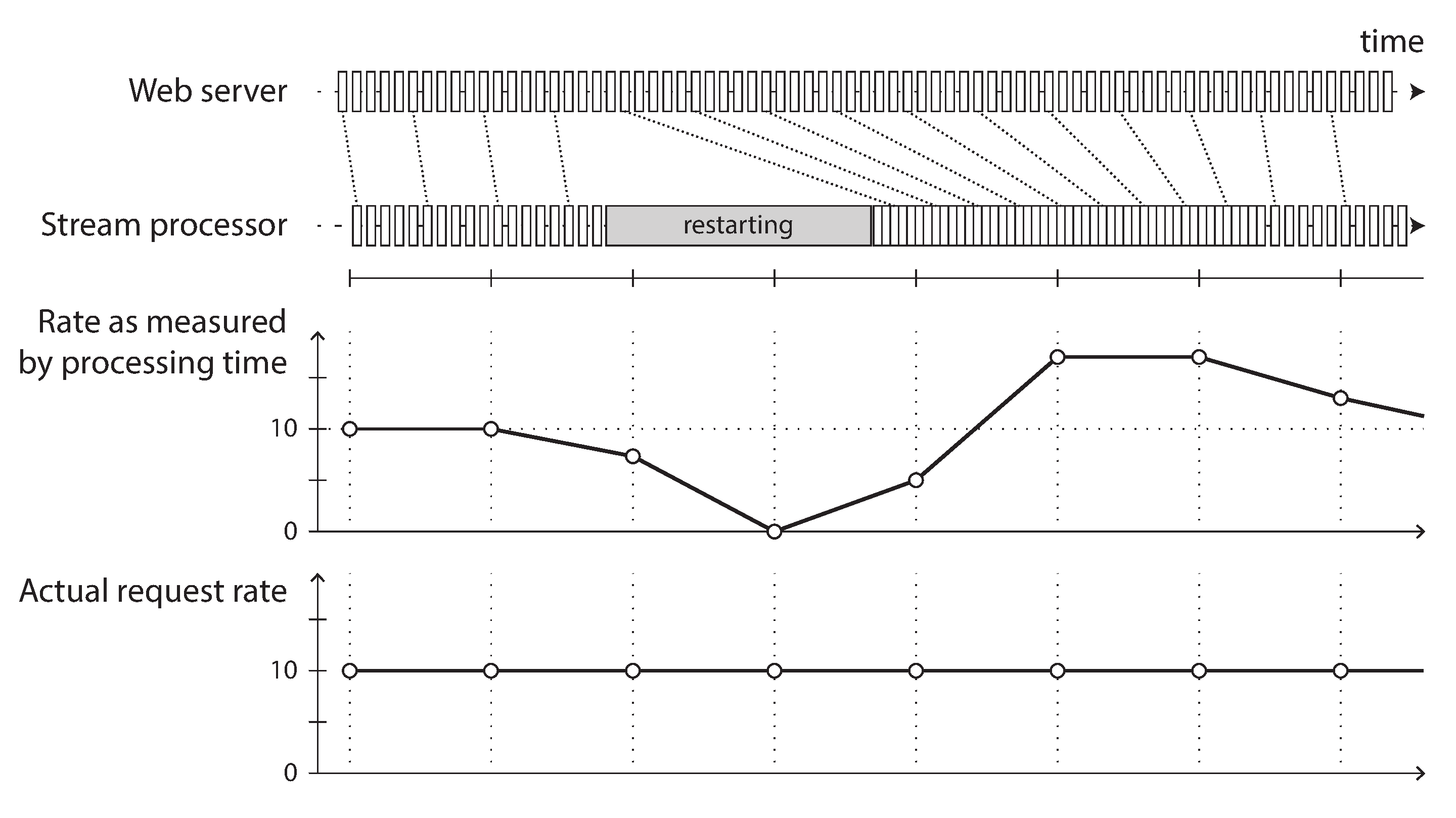
Figure 12-8 Windowing by processing time introduces artifacts due to variations in processing rate.

Handling straggler events

A tricky problem when defining windows in terms of event time is that you can never be sure when you have received all of the events for a particular window, or whether there are some events still to come.

For example, say you’re grouping events into one-minute windows so that you can count the number of requests per minute. You have counted some number of events with timestamps that fall in the 37th minute of the hour, and time has moved on; now most of the incoming events fall within the 38th and 39th minutes of the hour. When do you declare that you have finished the window for the 37th minute, and output its counter value?

You can time out and declare a window ready after you have not seen any new events for that window in a while. However, it could still happen that some events were buffered on another machine somewhere, delayed due to a network interruption. You need to be able to handle such straggler events that arrive after the window has already been declared complete. Broadly, you have two options ¹:

Ignore the straggler events, as they are probably a small percentage of events in normal circumstances. You can track the number of dropped events as a metric, and alert if you start dropping a significant amount of data.
Publish a correction, an updated value for the window with stragglers included. You may also need to retract the previous output.

In some cases it is possible to use a special message to indicate, “From now on there will be no more messages with a timestamp earlier than t,” which can be used by consumers to trigger windows ⁶⁶. However, if several producers on different machines are generating events, each with their own minimum timestamp thresholds, the consumers need to keep track of each producer individually. Adding and removing producers is trickier in this case.

Whose clock are you using, anyway?

Assigning timestamps to events is even more difficult when events can be buffered at several points in the system. For example, consider a mobile app that reports events for usage metrics to a server. The app may be used while the device is offline, in which case it will buffer events locally on the device and send them to a server when an internet connection is next available (which may be hours or even days later). To any consumers of this stream, the events will appear as extremely delayed stragglers.

In this context, the timestamp on the events should really be the time at which the user interaction occurred, according to the mobile device’s local clock. However, the clock on a user-controlled device often cannot be trusted, as it may be accidentally or deliberately set to the wrong time (see “Clock Synchronization and Accuracy”). The time at which the event was received by the server (according to the server’s clock) is more likely to be accurate, since the server is under your control, but less meaningful in terms of describing the user interaction.

To adjust for incorrect device clocks, one approach is to log three timestamps ⁶⁷:

The time at which the event occurred, according to the device clock
The time at which the event was sent to the server, according to the device clock
The time at which the event was received by the server, according to the server clock

By subtracting the second timestamp from the third, you can estimate the offset between the device clock and the server clock (assuming the network delay is negligible compared to the required timestamp accuracy). You can then apply that offset to the event timestamp, and thus estimate the true time at which the event actually occurred (assuming the device clock offset did not change between the time the event occurred and the time it was sent to the server).

This problem is not unique to stream processing—batch processing suffers from exactly the same issues of reasoning about time. It is just more noticeable in a streaming context, where we are more aware of the passage of time.

Types of windows

Once you know how the timestamp of an event should be determined, the next step is to decide how windows over time periods should be defined. The window can then be used for aggregations, for example to count events, or to calculate the average of values within the window. Several types of windows are in common use ⁶⁴, ⁶⁸:

Tumbling window: A tumbling window has a fixed length, and every event belongs to exactly one window. For example, if you have a 1-minute tumbling window, all the events with timestamps between 10:03:00 and 10:03:59 are grouped into one window, events between 10:04:00 and 10:04:59 into the next window, and so on. You could implement a 1-minute tumbling window by taking each event timestamp and rounding it down to the nearest minute to determine the window that it belongs to.
Hopping window: A hopping window also has a fixed length, but allows windows to overlap in order to provide some smoothing. For example, a 5-minute window with a hop size of 1 minute would contain the events between 10:03:00 and 10:07:59, then the next window would cover events between 10:04:00 and 10:08:59, and so on. You can implement this hopping window by first calculating 1-minute tumbling windows, and then aggregating over several adjacent windows.
Sliding window: A sliding window contains all the events that occur within some interval of each other. For example, a 5-minute sliding window would cover events at 10:03:39 and 10:08:12, because they are less than 5 minutes apart (note that tumbling and hopping 5-minute windows would not have put these two events in the same window, as they use fixed boundaries). A sliding window can be implemented by keeping a buffer of events sorted by time and removing old events when they expire from the window.
Session window: Unlike the other window types, a session window has no fixed duration. Instead, it is defined by grouping together all events for the same user that occur closely together in time, and the window ends when the user has been inactive for some time (for example, if there have been no events for 30 minutes). Sessionization is a common requirement for website analytics.

Window operations usually maintain temporary state. In some cases, the state is of a fixed size, no matter how large the window or how many events occur: for example, a counting operation will only have one counter regardless of the window size or event count. On the other hand, sliding windows or stream joins, which we discuss in the next section, require that events be buffered until the window finishes. Therefore, large window sizes or high-throughput streams can cause stream processors to keep a lot of temporary state. You must then take care to ensure the machines running stream processing tasks have enough capacity to maintain this state, whether in-memory or on-disk.

Stream Joins

In “JOIN and GROUP BY” we discussed how batch jobs can join datasets by key, and how such joins form an important part of data pipelines. Since stream processing generalizes data pipelines to incremental processing of unbounded datasets, there is exactly the same need for joins on streams.

However, the fact that new events can appear anytime on a stream makes joins on streams more challenging than in batch jobs. To understand the situation better, let’s distinguish three different types of joins: stream-stream joins, stream-table joins, and table-table joins. In the following sections we’ll illustrate each by example.

Stream-stream join (window join)

Say you have a search feature on your website, and you want to detect recent trends in searched-for URLs. Every time someone types a search query, you log an event containing the query and the results returned. Every time someone clicks one of the search results, you log another event recording the click. In order to calculate the click-through rate for each URL in the search results, you need to bring together the events for the search action and the click action, which are connected by having the same session ID. Similar analyses are needed in advertising systems ⁶⁹.

The click may never come if the user abandons their search, and even if it comes, the time between the search and the click may be highly variable: in many cases it might be a few seconds, but it could be as long as days or weeks (if a user runs a search, forgets about that browser tab, and then returns to the tab and clicks a result sometime later). Due to variable network delays, the click event may even arrive before the search event. You can choose a suitable window for the join—for example, you may choose to join a click with a search if they occur at most one hour apart.

Note that embedding the details of the search in the click event is not equivalent to joining the events: doing so would only tell you about the cases where the user clicked a search result, not about the searches where the user did not click any of the results. In order to measure search quality, you need accurate click-through rates, for which you need both the search events and the click events.

To implement this type of join, a stream processor needs to maintain state: for example, all the events that occurred in the last hour, indexed by session ID. Whenever a search event or click event occurs, it is added to the appropriate index, and the stream processor also checks the other index to see if another event for the same session ID has already arrived. If there is a matching event, you emit an event saying which search result was clicked. If the search event expires without you seeing a matching click event, you emit an event saying which search results were not clicked.

Stream-table join (stream enrichment)

In “JOIN and GROUP BY” (Figure 11-2) we saw an example of a batch job joining two datasets: a set of user activity events and a database of user profiles. It is natural to think of the user activity events as a stream, and to perform the same join on a continuous basis in a stream processor: the input is a stream of activity events containing a user ID, and the output is a stream of activity events in which the user ID has been augmented with profile information about the user. This process is sometimes known as enriching the activity events with information from the database.

To perform this join, the stream process needs to look at one activity event at a time, look up the event’s user ID in the database, and add the profile information to the activity event. The database lookup could be implemented by querying a remote database; however, as discussed in “JOIN and GROUP BY”, such remote queries are likely to be slow and risk overloading the database ⁵⁸.

Another approach is to load a copy of the database into the stream processor so that it can be queried locally without a network round-trip. This technique is called a hash join since the local copy of the database might be an in-memory hash table if it is small enough, or an index on the local disk.

The difference from batch jobs is that a batch job uses a point-in-time snapshot of the database as input, whereas a stream processor is long-running, and the contents of the database are likely to change over time, so the stream processor’s local copy of the database needs to be kept up to date. This issue can be solved by change data capture: the stream processor can subscribe to a changelog of the user profile database as well as the stream of activity events. When a profile is created or modified, the stream processor updates its local copy. Thus, we obtain a join between two streams: the activity events and the profile updates.

A stream-table join is actually very similar to a stream-stream join; the biggest difference is that for the table changelog stream, the join uses a window that reaches back to the “beginning of time” (a conceptually infinite window), with newer versions of records overwriting older ones. For the stream input, the join might not maintain a window at all.

Table-table join (materialized view maintenance)

Consider the social network timeline example that we discussed in “Case Study: Social Network Home Timelines”. We said that when a user wants to view their home timeline, it is too expensive to iterate over all the people the user is following, find their recent posts, and merge them.

Instead, we want a timeline cache: a kind of per-user “inbox” to which posts are written as they are sent, so that reading the timeline is a single lookup. Materializing and maintaining this cache requires the following event processing:

When user u sends a new post, it is added to the timeline of every user who is following u.
When a user deletes a post, or deletes their entire account, it is removed from all users' timelines.
When user u₁ starts following user u₂, recent posts by u₂ are added to u₁’s timeline.
When user u₁ unfollows user u₂, posts by u₂ are removed from u₁’s timeline.

To implement this cache maintenance in a stream processor, you need streams of events for posts (sending and deleting) and for follow relationships (following and unfollowing). The stream process needs to maintain a database containing the set of followers for each user so that it knows which timelines need to be updated when a new post arrives.

Another way of looking at this stream process is that it maintains a materialized view for a query that joins two tables (posts and follows), something like the following:

SELECT follows.follower_id AS timeline_id,
  array_agg(posts.* ORDER BY posts.timestamp DESC)
FROM posts
JOIN follows ON follows.followee_id = posts.sender_id
GROUP BY follows.follower_id

The join of the streams corresponds directly to the join of the tables in that query. The timelines are effectively a cache of the result of this query, updated every time the underlying tables change.

Note

If you regard a stream as the derivative of a table, as in Figure 12-7, and regard a join as a product of two tables u·v, something interesting happens: the stream of changes to the materialized join follows the product rule (u·v)′ = u′v + uv′. In words: any change of posts is joined with the current followers, and any change of followers is joined with the current posts ³⁷.

Time-dependence of joins

The three types of joins described here (stream-stream, stream-table, and table-table) have a lot in common: they all require the stream processor to maintain some state (search and click events, user profiles, or follower list) based on one join input, and query that state on messages from the other join input.

The order of the events that maintain the state is important (it matters whether you first follow and then unfollow, or the other way round). In a sharded event log like Kafka, the ordering of events within a single shard (partition) is preserved, but there is typically no ordering guarantee across different streams or shards.

This raises a question: if events on different streams happen around a similar time, in which order are they processed? In the stream-table join example, if a user updates their profile, which activity events are joined with the old profile (processed before the profile update), and which are joined with the new profile (processed after the profile update)? Put another way: if state changes over time, and you join with some state, what point in time do you use for the join?

Such time dependence can occur in many places. For example, if you sell things, you need to apply the right tax rate to invoices, which depends on the country or state, the type of product, and the date of sale (since tax rates change from time to time). When joining sales to a table of tax rates, you probably want to join with the tax rate at the time of the sale, which may be different from the current tax rate if you are reprocessing historical data.

If the ordering of events across streams is undetermined, the join becomes nondeterministic ⁷⁰, which means you cannot rerun the same job on the same input and necessarily get the same result: the events on the input streams may be interleaved in a different way when you run the job again.

In data warehouses, this issue is known as a slowly changing dimension (SCD), and it is often addressed by using a unique identifier for a particular version of the joined record: for example, every time the tax rate changes, it is given a new identifier, and the invoice includes the identifier for the tax rate at the time of sale ⁷¹, ⁷². This change makes the join deterministic, but has the consequence that log compaction is not possible, since all versions of the records in the table need to be retained. Alternatively, you can denormalize the data and include the applicable tax rate directly in every sale event.

Fault Tolerance

In the final section of this chapter, let’s consider how stream processors can tolerate faults. We saw in Chapter 11 that batch processing frameworks can tolerate faults fairly easily: if a task fails, it can simply be started again on another machine, and the output of the failed task is discarded. This transparent retry is possible because input files are immutable, each task writes its output to a separate file, and output is only made visible when a task completes successfully.

In particular, the batch approach to fault tolerance ensures that the output of the batch job is the same as if nothing had gone wrong, even if in fact some tasks did fail. It appears as though every input record was processed exactly once—no records are skipped, and none are processed twice. Although restarting tasks means that records may in fact be processed multiple times, the visible effect in the output is as if they had only been processed once. This principle is known as exactly-once semantics, although effectively-once would be a more descriptive term ⁷³.

The same issue of fault tolerance arises in stream processing, but it is less straightforward to handle: waiting until a task is finished before making its output visible is not an option, because a stream is infinite and so you can never finish processing it.

Microbatching and checkpointing

One solution is to break the stream into small blocks, and treat each block like a miniature batch process. This approach is called microbatching, and it is used in Spark Streaming ⁷⁴. The batch size is typically around one second, which is the result of a performance compromise: smaller batches incur greater scheduling and coordination overhead, while larger batches mean a longer delay before results of the stream processor become visible.

Microbatching also implicitly provides a tumbling window equal to the batch size (windowed by processing time, not event timestamps); any jobs that require larger windows need to explicitly carry over state from one microbatch to the next.

A variant approach, used in Apache Flink, is to periodically generate rolling checkpoints of state and write them to durable storage ⁷⁵, ⁷⁶. If a stream operator crashes, it can restart from its most recent checkpoint and discard any output generated between the last checkpoint and the crash. The checkpoints are triggered by barriers in the message stream, similar to the boundaries between microbatches, but without forcing a particular window size.

Within the confines of the stream processing framework, the microbatching and checkpointing approaches provide the same exactly-once semantics as batch processing. However, as soon as output leaves the stream processor (for example, by writing to a database, sending messages to an external message broker, or sending emails), the framework is no longer able to discard the output of a failed microbatch. In this case, restarting a failed task causes the external side effect to happen twice, and microbatching or checkpointing alone is not sufficient to prevent this problem.

Atomic commit revisited

In order to give the appearance of exactly-once processing in the presence of faults, we need to ensure that all outputs and side effects of processing an event take effect if and only if the processing is successful. Those effects include any messages sent to downstream operators or external messaging systems (including email or push notifications), any database writes, any changes to operator state, and any acknowledgment of input messages (including moving the consumer offset forward in a log-based message broker).

Those things either all need to happen atomically, or none of them must happen, but they should not go out of sync with each other. If this approach sounds familiar, it is because we discussed it in “Exactly-once message processing” in the context of distributed transactions and two-phase commit.

In Chapter 8 we discussed the problems in the traditional implementations of distributed transactions, such as XA. However, in more restricted environments it is possible to implement such an atomic commit facility efficiently. This approach is used in Google Cloud Dataflow ⁶⁶, ⁷⁵, VoltDB ⁷⁷, and Apache Kafka ⁷⁸, ⁷⁹. Unlike XA, these implementations do not attempt to provide transactions across heterogeneous technologies, but instead keep the transactions internal by managing both state changes and messaging within the stream processing framework. The overhead of the transaction protocol can be amortized by processing several input messages within a single transaction.

Idempotence

Our goal is to discard the partial output of any failed tasks so that they can be safely retried without taking effect twice. Distributed transactions are one way of achieving that goal, but another way is to rely on idempotence, as we saw in “Durable Execution and Workflows” ⁸⁰.

An idempotent operation is one that you can perform multiple times, and it has the same effect as if you performed it only once. For example, deleting a key in a key-value store is idempotent (deleting the value again has no further effect), whereas incrementing a counter is not idempotent (performing the increment again means the value is incremented twice).

Even if an operation is not naturally idempotent, it can often be made idempotent with a bit of extra metadata. For example, when consuming messages from Kafka, every message has a persistent, monotonically increasing offset. When writing a value to an external database, you can include the offset of the message that triggered the last write with the value. Thus, you can tell whether an update has already been applied, and avoid performing the same update again.

The state handling in Storm’s Trident is based on a similar idea. Relying on idempotence implies several assumptions: restarting a failed task must replay the same messages in the same order (a log-based message broker does this), the processing must be deterministic, and no other node may concurrently update the same value ⁸¹, ⁸².

When failing over from one processing node to another, fencing may be required (see “Distributed Locks and Leases”) to prevent interference from a node that is thought to be dead but is actually alive. Despite all those caveats, idempotent operations can be an effective way of achieving exactly-once semantics with only a small overhead.

Rebuilding state after a failure

Any stream process that requires state—for example, any windowed aggregations (such as counters, averages, and histograms) and any tables and indexes used for joins—must ensure that this state can be recovered after a failure.

One option is to keep the state in a remote datastore and replicate it, although having to query a remote database for each individual message can be slow. An alternative is to keep state local to the stream processor, and replicate it periodically. Then, when the stream processor is recovering from a failure, the new task can read the replicated state and resume processing without data loss.

For example, Flink periodically captures snapshots of operator state and writes them to durable storage such as a distributed filesystem ⁷⁵, ⁷⁶, and Kafka Streams replicates state changes by sending them to a dedicated Kafka topic with log compaction, similar to change data capture ⁸³. VoltDB replicates state by redundantly processing each input message on several nodes (see “Actual Serial Execution”).

In some cases, it may not even be necessary to replicate the state, because it can be rebuilt from the input streams. For example, if the state consists of aggregations over a fairly short window, it may be fast enough to simply replay the input events corresponding to that window. If the state is a local replica of a database, maintained by change data capture, the database can also be rebuilt from the log-compacted change stream.

However, all of these trade-offs depend on the performance characteristics of the underlying infrastructure: in some systems, network delay may be lower than disk access latency, and network bandwidth may be comparable to disk bandwidth. There is no universally ideal trade-off for all situations, and the merits of local versus remote state may also shift as storage and networking technologies evolve.

Summary

In this chapter we have discussed event streams, what purposes they serve, and how to process them. In some ways, stream processing is very much like the batch processing we discussed in Chapter 11, but done continuously on unbounded (never-ending) streams rather than on a fixed-size input ⁸⁴. From this perspective, message brokers and event logs serve as the streaming equivalent of a filesystem.

We spent some time comparing two types of message brokers:

AMQP/JMS-style message broker: The broker assigns individual messages to consumers, and consumers acknowledge individual messages when they have been successfully processed. Messages are deleted from the broker once they have been acknowledged. This approach is appropriate as an asynchronous form of RPC (see also “Event-Driven Architectures”), for example in a task queue, where the exact order of message processing is not important and where there is no need to go back and read old messages again after they have been processed.
Log-based message broker: The broker assigns all messages in a shard to the same consumer node, and always delivers messages in the same order. Parallelism is achieved through sharding, and consumers track their progress by checkpointing the offset of the last message they have processed. The broker retains messages on disk, so it is possible to jump back and reread old messages if necessary.

The log-based approach has similarities to the replication logs found in databases (see Chapter 6) and log-structured storage engines (see Chapter 4). It is also a form of consensus, as we saw in Chapter 10. We saw that this approach is especially appropriate for stream processing systems that consume input streams and generate derived state or derived output streams.

In terms of where streams come from, we discussed several possibilities: user activity events, sensors providing periodic readings, and data feeds (e.g., market data in finance) are naturally represented as streams. We saw that it can also be useful to think of the writes to a database as a stream: we can capture the changelog—i.e., the history of all changes made to a database—either implicitly through change data capture or explicitly through event sourcing. Log compaction allows the stream to retain a full copy of the contents of a database.

Representing databases as streams opens up powerful opportunities for integrating systems. You can keep derived data systems such as search indexes, caches, and analytics systems continually up to date by consuming the log of changes and applying them to the derived system. You can even build fresh views onto existing data by starting from scratch and consuming the log of changes from the beginning all the way to the present.

The facilities for maintaining state as streams and replaying messages are also the basis for the techniques that enable stream joins and fault tolerance in various stream processing frameworks. We discussed several purposes of stream processing, including searching for event patterns (complex event processing), computing windowed aggregations (stream analytics), and keeping derived data systems up to date (materialized views).

We then discussed the difficulties of reasoning about time in a stream processor, including the distinction between processing time and event timestamps, and the problem of dealing with straggler events that arrive after you thought your window was complete.

We distinguished three types of joins that may appear in stream processes:

Stream-stream joins: Both input streams consist of activity events, and the join operator searches for related events that occur within some window of time. For example, it may match two actions taken by the same user within 30 minutes of each other. The two join inputs may in fact be the same stream (a self-join) if you want to find related events within that one stream.
Stream-table joins: One input stream consists of activity events, while the other is a database changelog. The changelog keeps a local copy of the database up to date. For each activity event, the join operator queries the database and outputs an enriched activity event.
Table-table joins: Both input streams are database changelogs. In this case, every change on one side is joined with the latest state of the other side. The result is a stream of changes to the materialized view of the join between the two tables.

Finally, we discussed techniques for achieving fault tolerance and exactly-once semantics in a stream processor. As with batch processing, we need to discard the partial output of any failed tasks. However, since a stream process is long-running and produces output continuously, we can’t simply discard all output. Instead, a finer-grained recovery mechanism can be used, based on microbatching, checkpointing, transactions, or idempotent writes.

Footnotes

References

Tyler Akidau, Robert Bradshaw, Craig Chambers, Slava Chernyak, Rafael J. Fernández-Moctezuma, Reuven Lax, Sam McVeety, Daniel Mills, Frances Perry, Eric Schmidt, and Sam Whittle. The Dataflow Model: A Practical Approach to Balancing Correctness, Latency, and Cost in Massive-Scale, Unbounded, Out-of-Order Data Processing. Proceedings of the VLDB Endowment, volume 8, issue 12, pages 1792–1803, August 2015. doi:10.14778/2824032.2824076 ↩︎ ↩︎
Harold Abelson, Gerald Jay Sussman, and Julie Sussman. Structure and Interpretation of Computer Programs, 2nd edition. MIT Press, 1996. ISBN: 978-0-262-51087-5, archived at archive.org/details/sicp_20211010 ↩︎
Patrick Th. Eugster, Pascal A. Felber, Rachid Guerraoui, and Anne-Marie Kermarrec. The Many Faces of Publish/Subscribe. ACM Computing Surveys, volume 35, issue 2, pages 114–131, June 2003. doi:10.1145/857076.857078 ↩︎
Don Carney, Uğur Çetintemel, Mitch Cherniack, Christian Convey, Sangdon Lee, Greg Seidman, Michael Stonebraker, Nesime Tatbul, and Stan Zdonik. Monitoring Streams – A New Class of Data Management Applications. At 28th International Conference on Very Large Data Bases (VLDB), August 2002. doi:10.1016/B978-155860869-6/50027-5 ↩︎
Matthew Sackman. Pushing Back. wellquite.org, May 2016. Archived at perma.cc/3KCZ-RUFY ↩︎ ↩︎
Thomas Figg (tef). how (not) to write a pipeline. cohost.org, June 2023. Archived at perma.cc/A3V8-NYCM ↩︎
Vicent Martí. Brubeck, a statsd-Compatible Metrics Aggregator. github.blog, June 2015. Archived at perma.cc/TP3Q-DJYM ↩︎
Seth Lowenberger. MoldUDP64 Protocol Specification V 1.00. nasdaqtrader.com, July 2009. Archived at https://perma.cc/7CRQ-QBD7 ↩︎
Ian Malpass. Measure Anything, Measure Everything. codeascraft.com, February 2011. Archived at archive.org ↩︎
Dieter Plaetinck. 25 Graphite, Grafana and statsd Gotchas. grafana.com, March 2016. Archived at perma.cc/3NP3-67U7 ↩︎
Jeff Lindsay. Web Hooks to Revolutionize the Web. progrium.com, May 2007. Archived at perma.cc/BF9U-XNX4 ↩︎
Jim N. Gray. Queues Are Databases. Microsoft Research Technical Report MSR-TR-95-56, December 1995. Archived at arxiv.org ↩︎
Mark Hapner, Rich Burridge, Rahul Sharma, Joseph Fialli, Kate Stout, and Nigel Deakin. JSR-343 Java Message Service (JMS) 2.0 Specification. jms-spec.java.net, March 2013. Archived at perma.cc/E4YG-46TA ↩︎
Sanjay Aiyagari, Matthew Arrott, Mark Atwell, Jason Brome, Alan Conway, Robert Godfrey, Robert Greig, Pieter Hintjens, John O’Hara, Matthias Radestock, Alexis Richardson, Martin Ritchie, Shahrokh Sadjadi, Rafael Schloming, Steven Shaw, Martin Sustrik, Carl Trieloff, Kim van der Riet, and Steve Vinoski. AMQP: Advanced Message Queuing Protocol Specification. Version 0-9-1, November 2008. Archived at perma.cc/6YJJ-GM9X ↩︎
Architectural overview of Pub/Sub. cloud.google.com, 2025. Archived at perma.cc/VWF5-ABP4 ↩︎ ↩︎
Aris Tzoumas. Lessons from scaling PostgreSQL queues to 100k events per second. rudderstack.com, July 2025. Archived at perma.cc/QD8C-VA4Y ↩︎
Robin Moffatt. Kafka Connect Deep Dive – Error Handling and Dead Letter Queues. confluent.io, March 2019. Archived at perma.cc/KQ5A-AB28 ↩︎
Dunith Danushka. Message reprocessing: How to implement the dead letter queue. redpanda.com. Archived at perma.cc/R7UB-WEWF ↩︎
Damien Gasparina, Loic Greffier, and Sebastien Viale. KIP-1034: Dead letter queue in Kafka Streams. cwiki.apache.org, April 2024. Archived at perma.cc/3VXV-QXAN ↩︎
Jay Kreps, Neha Narkhede, and Jun Rao. Kafka: A Distributed Messaging System for Log Processing. At 6th International Workshop on Networking Meets Databases (NetDB), June 2011. Archived at perma.cc/CSW7-TCQ5 ↩︎
Jay Kreps. Benchmarking Apache Kafka: 2 Million Writes Per Second (On Three Cheap Machines). engineering.linkedin.com, April 2014. Archived at archive.org ↩︎
Kartik Paramasivam. How We’re Improving and Advancing Kafka at LinkedIn. engineering.linkedin.com, September 2015. Archived at perma.cc/3S3V-JCYJ ↩︎
Philippe Dobbelaere and Kyumars Sheykh Esmaili. Kafka versus RabbitMQ: A comparative study of two industry reference publish/subscribe implementations. At 11th ACM International Conference on Distributed and Event-based Systems (DEBS), June 2017. doi:10.1145/3093742.3093908 ↩︎
Kate Holterhoff. Why Message Queues Endure: A History. redmonk.com, December 2024. Archived at perma.cc/6DX8-XK4W ↩︎
Andrew Schofield. KIP-932: Queues for Kafka. cwiki.apache.org, May 2023. Archived at perma.cc/LBE4-BEMK ↩︎
Jack Vanlightly. The advantages of queues on logs. jack-vanlightly.com, October 2023. Archived at perma.cc/WJ7V-287K ↩︎
Jay Kreps. The Log: What Every Software Engineer Should Know About Real-Time Data’s Unifying Abstraction. engineering.linkedin.com, December 2013. Archived at perma.cc/2JHR-FR64 ↩︎ ↩︎
Andy Hattemer. Change Data Capture is having a moment. Why? materialize.com, September 2021. Archived at perma.cc/AL37-P53C ↩︎
Prem Santosh Udaya Shankar. Streaming MySQL Tables in Real-Time to Kafka. engineeringblog.yelp.com, August 2016. Archived at perma.cc/5ZR3-2GVV ↩︎
Andreas Andreakis, Ioannis Papapanagiotou. DBLog: A Watermark Based Change-Data-Capture Framework. October 2020. Archived at arxiv.org ↩︎
Jiri Pechanec. Percolator. debezium.io, October 2021. Archived at perma.cc/EQ8E-W6KQ ↩︎
Debezium maintainers. Debezium Connector for Cassandra. debezium.io. Archived at perma.cc/WR6K-EKMD ↩︎
Neha Narkhede. Announcing Kafka Connect: Building Large-Scale Low-Latency Data Pipelines. confluent.io, February 2016. Archived at perma.cc/8WXJ-L6GF ↩︎ ↩︎
Chris Riccomini. Kafka change data capture breaks database encapsulation. cnr.sh, November 2018. Archived at perma.cc/P572-9MKF ↩︎
Gunnar Morling. “Change Data Capture Breaks Encapsulation”. Does it, though? decodable.co, November 2023. Archived at perma.cc/YX2P-WNWR ↩︎
Gunnar Morling. Revisiting the Outbox Pattern. decodable.co, October 2024. Archived at perma.cc/M5ZL-RPS9 ↩︎
Ashish Gupta and Inderpal Singh Mumick. Maintenance of Materialized Views: Problems, Techniques, and Applications. IEEE Data Engineering Bulletin, volume 18, issue 2, pages 3–18, June 1995. Archived at archive.org ↩︎ ↩︎ ↩︎
Mihai Budiu, Tej Chajed, Frank McSherry, Leonid Ryzhyk, Val Tannen. DBSP: Incremental Computation on Streams and Its Applications to Databases. SIGMOD Record, volume 53, issue 1, pages 87–95, March 2024. doi:10.1145/3665252.3665271 ↩︎ ↩︎
Jim Gray and Andreas Reuter. Transaction Processing: Concepts and Techniques. Morgan Kaufmann, 1992. ISBN: 9781558601901 ↩︎
Martin Kleppmann. Accounting for Computer Scientists. martin.kleppmann.com, March 2011. Archived at perma.cc/9EGX-P38N ↩︎
Pat Helland. Immutability Changes Everything. At 7th Biennial Conference on Innovative Data Systems Research (CIDR), January 2015. ↩︎ ↩︎
Martin Kleppmann. Making Sense of Stream Processing. Report, O’Reilly Media, May 2016. Archived at perma.cc/RAY4-JDVX ↩︎
Kartik Paramasivam. Stream Processing Hard Problems – Part 1: Killing Lambda. engineering.linkedin.com, June 2016. Archived at archive.org ↩︎
Stéphane Derosiaux. CQRS: What? Why? How? sderosiaux.medium.com, September 2019. Archived at perma.cc/FZ3U-HVJ4 ↩︎
Baron Schwartz. Immutability, MVCC, and Garbage Collection. xaprb.com, December 2013. Archived at archive.org ↩︎
Daniel Eloff, Slava Akhmechet, Jay Kreps, et al. Re: Turning the Database Inside-out with Apache Samza. Hacker News discussion, news.ycombinator.com, March 2015. Archived at perma.cc/ML9E-JC83 ↩︎
Datomic Documentation: Excision. Cognitect, Inc., docs.datomic.com. Archived at perma.cc/J5QQ-SH32 ↩︎
Fossil Documentation: Deleting Content from Fossil. fossil-scm.org, 2025. Archived at perma.cc/DS23-GTNG ↩︎
Jay Kreps. The irony of distributed systems is that data loss is really easy but deleting data is surprisingly hard. x.com, March 2015. Archived at perma.cc/7RRZ-V7B7 ↩︎
Brent Robinson. Crypto shredding: How it can solve modern data retention challenges. medium.com, January 2019. Archived at https://perma.cc/4LFK-S6XE ↩︎
Matthew D. Green and Ian Miers. Forward Secure Asynchronous Messaging from Puncturable Encryption. At IEEE Symposium on Security and Privacy, May 2015. doi:10.1109/SP.2015.26 ↩︎
David C. Luckham. What’s the Difference Between ESP and CEP? complexevents.com, June 2019. Archived at perma.cc/E7PZ-FDEF ↩︎
Arvind Arasu, Shivnath Babu, and Jennifer Widom. The CQL Continuous Query Language: Semantic Foundations and Query Execution. The VLDB Journal, volume 15, issue 2, pages 121–142, June 2006. doi:10.1007/s00778-004-0147-z ↩︎
Julian Hyde. Data in Flight: How Streaming SQL Technology Can Help Solve the Web 2.0 Data Crunch. ACM Queue, volume 7, issue 11, December 2009. doi:10.1145/1661785.1667562 ↩︎
Philippe Flajolet, Éric Fusy, Olivier Gandouet, and Frédéric Meunier. HyperLogLog: The Analysis of a Near-Optimal Cardinality Estimation Algorithm. At Conference on Analysis of Algorithms (AofA), June 2007. doi:10.46298/dmtcs.3545 ↩︎
Jay Kreps. Questioning the Lambda Architecture. oreilly.com, July 2014. Archived at perma.cc/2WY5-HC8Y ↩︎
Ian Reppel. An Overview of Apache Streaming Technologies. ianreppel.org, March 2016. Archived at perma.cc/BB3E-QJLW ↩︎
Jay Kreps. Why Local State is a Fundamental Primitive in Stream Processing. oreilly.com, July 2014. Archived at perma.cc/P8HU-R5LA ↩︎ ↩︎
RisingWave Labs. Deep Dive Into the RisingWave Stream Processing Engine - Part 2: Computational Model. risingwave.com, November 2023. Archived at perma.cc/LM74-XDEL ↩︎
Frank McSherry, Derek G. Murray, Rebecca Isaacs, and Michael Isard. Differential dataflow. At 6th Biennial Conference on Innovative Data Systems Research (CIDR), January 2013. ↩︎
Andy Hattemer. Incremental Computation in the Database. materialize.com, March 2020. Archived at perma.cc/AL94-YVRN ↩︎
Shay Banon. Percolator. elastic.co, February 2011. Archived at perma.cc/LS5R-4FQX ↩︎
Alan Woodward and Martin Kleppmann. Real-Time Full-Text Search with Luwak and Samza. martin.kleppmann.com, April 2015. Archived at perma.cc/2U92-Q7R4 ↩︎
Tyler Akidau. The World Beyond Batch: Streaming 102. oreilly.com, January 2016. Archived at perma.cc/4XF9-8M2K ↩︎ ↩︎
Stephan Ewen. Streaming Analytics with Apache Flink. At Kafka Summit, April 2016. Archived at perma.cc/QBQ4-F9MR ↩︎
Tyler Akidau, Alex Balikov, Kaya Bekiroğlu, Slava Chernyak, Josh Haberman, Reuven Lax, Sam McVeety, Daniel Mills, Paul Nordstrom, and Sam Whittle. MillWheel: Fault-Tolerant Stream Processing at Internet Scale. Proceedings of the VLDB Endowment, volume 6, issue 11, pages 1033–1044, August 2013. doi:10.14778/2536222.2536229 ↩︎ ↩︎
Alex Dean. Improving Snowplow’s Understanding of Time. snowplow.io, September 2015. Archived at perma.cc/6CT9-Z3Q2 ↩︎
Azure Stream Analytics: Windowing functions. Microsoft Azure Reference, learn.microsoft.com, July 2025. Archived at archive.org ↩︎
Rajagopal Ananthanarayanan, Venkatesh Basker, Sumit Das, Ashish Gupta, Haifeng Jiang, Tianhao Qiu, Alexey Reznichenko, Deomid Ryabkov, Manpreet Singh, and Shivakumar Venkataraman. Photon: Fault-Tolerant and Scalable Joining of Continuous Data Streams. At ACM International Conference on Management of Data (SIGMOD), June 2013. doi:10.1145/2463676.2465272 ↩︎
Ben Kirwin. Doing the Impossible: Exactly-Once Messaging Patterns in Kafka. ben.kirw.in, November 2014. Archived at perma.cc/A5QL-QRX7 ↩︎
Pat Helland. Data on the Outside Versus Data on the Inside. At 2nd Biennial Conference on Innovative Data Systems Research (CIDR), January 2005. ↩︎
Ralph Kimball and Margy Ross. The Data Warehouse Toolkit: The Definitive Guide to Dimensional Modeling, 3rd edition. John Wiley & Sons, 2013. ISBN: 978-1-118-53080-1 ↩︎
Viktor Klang. I’m coining the phrase ’effectively-once’ for message processing with at-least-once + idempotent operations. x.com, October 2016. Archived at perma.cc/7DT9-TDG2 ↩︎
Matei Zaharia, Tathagata Das, Haoyuan Li, Scott Shenker, and Ion Stoica. Discretized Streams: An Efficient and Fault-Tolerant Model for Stream Processing on Large Clusters. At 4th USENIX Conference in Hot Topics in Cloud Computing (HotCloud), June 2012. ↩︎
Kostas Tzoumas, Stephan Ewen, and Robert Metzger. High-Throughput, Low-Latency, and Exactly-Once Stream Processing with Apache Flink. ververica.com, August 2015. Archived at archive.org ↩︎ ↩︎ ↩︎
Paris Carbone, Gyula Fóra, Stephan Ewen, Seif Haridi, and Kostas Tzoumas. Lightweight Asynchronous Snapshots for Distributed Dataflows. arXiv:1506.08603 [cs.DC], June 2015. ↩︎ ↩︎
Ryan Betts and John Hugg. Fast Data: Smart and at Scale. Report, O’Reilly Media, October 2015. Archived at perma.cc/VQ6S-XQQY ↩︎
Neha Narkhede and Guozhang Wang. Exactly-Once Semantics Are Possible: Here’s How Kafka Does It. confluent.io, June 2019. Archived at perma.cc/Q2AU-Q2ED ↩︎
Jason Gustafson, Flavio Junqueira, Apurva Mehta, Sriram Subramanian, and Guozhang Wang. KIP-98 – Exactly Once Delivery and Transactional Messaging. cwiki.apache.org, November 2016. Archived at perma.cc/95PT-RCTG ↩︎
Pat Helland. Idempotence Is Not a Medical Condition. Communications of the ACM, volume 55, issue 5, page 56, May 2012. doi:10.1145/2160718.2160734 ↩︎
Jay Kreps. Re: Trying to Achieve Deterministic Behavior on Recovery/Rewind. Email to samza-dev mailing list, September 2014. Archived at perma.cc/7DPD-GJNL ↩︎
E. N. (Mootaz) Elnozahy, Lorenzo Alvisi, Yi-Min Wang, and David B. Johnson. A Survey of Rollback-Recovery Protocols in Message-Passing Systems. ACM Computing Surveys, volume 34, issue 3, pages 375–408, September 2002. doi:10.1145/568522.568525 ↩︎
Adam Warski. Kafka Streams – How Does It Fit the Stream Processing Landscape? softwaremill.com, June 2016. Archived at perma.cc/WQ5Q-H2J2 ↩︎
Stephan Ewen, Fabian Hueske, and Xiaowei Jiang. Batch as a Special Case of Streaming and Alibaba’s contribution of Blink. flink.apache.org, February 2019. Archived at perma.cc/A529-SKA9 ↩︎

13. A Philosophy of Streaming Systems

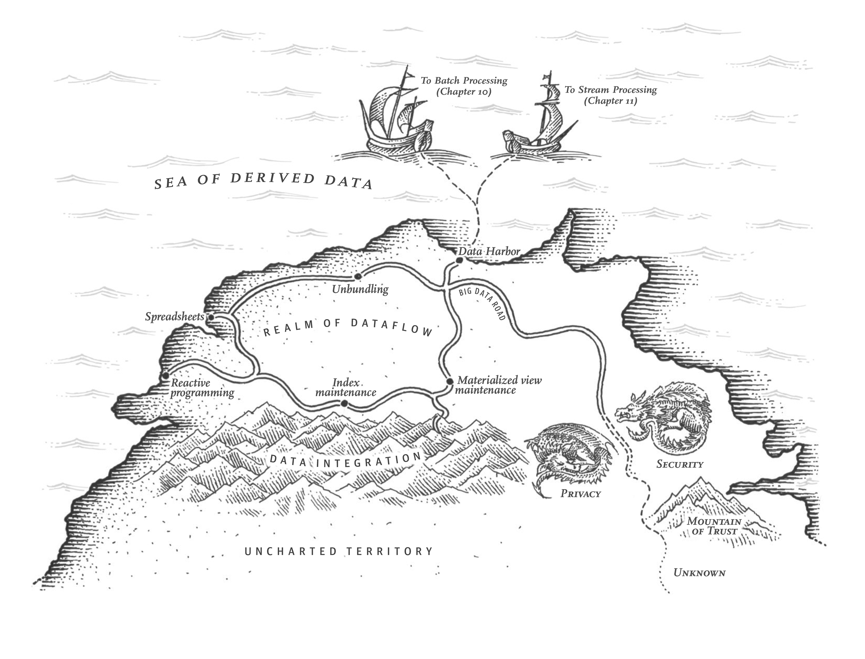
If a thing be ordained to another as to its end, its last end cannot consist in the preservation of its being. Hence a captain does not intend as a last end, the preservation of the ship entrusted to him, since a ship is ordained to something else as its end, viz. to navigation.

(Often quoted as: If the highest aim of a captain was the preserve his ship, he would keep it in port forever.)

St. Thomas Aquinas, Summa Theologica (1265–1274)

A NOTE FOR EARLY RELEASE READERS

This will be the 13th chapter of the final book. The GitHub repo for this book is https://github.com/ept/ddia2-feedback.

If you’d like to be actively involved in reviewing and commenting on this draft, please reach out on GitHub.

In Chapter 2 we discussed the goal of creating applications and systems that are reliable, scalable, and maintainable. These themes have run through all of the chapters: for example, we discussed many fault-tolerance algorithms that help improve reliability, sharding to improve scalability, and mechanisms for evolution and abstraction that improve maintainability.

In this chapter we will bring all of these ideas together, and build on the streaming/event-driven architecture ideas from Chapter 12 in particular to develop a philosophy of application development that meets those goals. This chapter is more opinionated than previous chapters, presenting a deep-dive into one particular philosophy rather than comparing multiple approaches.

Data Integration

A recurring theme in this book has been that for any given problem, there are several solutions, all of which have different pros, cons, and trade-offs. For example, when discussing storage engines in Chapter 4, we saw log-structured storage, B-trees, and column-oriented storage. When discussing replication in Chapter 6, we saw single-leader, multi-leader, and leaderless approaches.

If you have a problem such as “I want to store some data and look it up again later,” there is no one right solution, but many different approaches that are each appropriate in different circumstances. A software implementation typically has to pick one particular approach. It’s hard enough to get one code path robust and performing well—trying to do everything in one piece of software almost guarantees that the implementation will be poor.

Thus, the most appropriate choice of software tool also depends on the circumstances. Every piece of software, even a so-called “general-purpose” database, is designed for a particular usage pattern.

Faced with this profusion of alternatives, the first challenge is then to figure out the mapping between the software products and the circumstances in which they are a good fit. Vendors are understandably reluctant to tell you about the kinds of workloads for which their software is poorly suited, but hopefully the previous chapters have equipped you with some questions to ask in order to read between the lines and better understand the trade-offs.

However, even if you perfectly understand the mapping between tools and circumstances for their use, there is another challenge: in complex applications, data is often used in several different ways. There is unlikely to be one piece of software that is suitable for all the different circumstances in which the data is used, so you inevitably end up having to cobble together several different pieces of software in order to provide your application’s functionality.

Combining Specialized Tools by Deriving Data

For example, it is common to need to integrate an OLTP database with a full-text search index in order to handle queries for arbitrary keywords. Although some databases (such as PostgreSQL) include a full-text indexing feature, which can be sufficient for simple applications ¹, more sophisticated search facilities require specialist information retrieval tools. Conversely, search indexes are generally not very suitable as a durable system of record, and so many applications need to combine two different tools in order to satisfy all of the requirements.

We touched on the issue of integrating data systems in “Keeping Systems in Sync”. As the number of different representations of the data increases, the integration problem becomes harder. Besides the database and the search index, perhaps you need to keep copies of the data in analytics systems (data warehouses, or batch and stream processing systems); maintain caches or denormalized versions of objects that were derived from the original data; pass the data through machine learning, classification, ranking, or recommendation systems; or send notifications based on changes to the data.

Reasoning about dataflows

When copies of the same data need to be maintained in several storage systems in order to satisfy different access patterns, you need to be very clear about the inputs and outputs: where is data written first, and which representations are derived from which sources? How do you get data into all the right places, in the right formats?

For example, you might arrange for data to first be written to a system of record database, capturing the changes made to that database (see “Change Data Capture”) and then applying the changes to the search index in the same order. If change data capture (CDC) is the only way of updating the index, you can be confident that the index is entirely derived from the system of record, and therefore consistent with it (barring bugs in the software). Writing to the database is the only way of supplying new input into this system.

Allowing the application to directly write to both the search index and the database introduces the problem shown in Figure 12-4, in which two clients concurrently send conflicting writes, and the two storage systems process them in a different order. In this case, neither the database nor the search index is “in charge” of determining the order of writes, and so they may make contradictory decisions and become permanently inconsistent with each other.

If it is possible for you to funnel all user input through a single system that decides on an ordering for all writes, it becomes much easier to derive other representations of the data by processing the writes in the same order. This is an application of the state machine replication approach that we saw in “Consensus in Practice”. Whether you use change data capture or an event sourcing log is less important than simply the principle of deciding on a total order.

Updating a derived data system based on an event log can often be made deterministic and idempotent (see “Idempotence”), making it quite easy to recover from faults.

Derived data versus distributed transactions

The classic approach for keeping different data systems consistent with each other involves distributed transactions, as discussed in “Two-Phase Commit (2PC)”. How does the approach of using derived data systems fare in comparison to distributed transactions?

At an abstract level, they achieve a similar goal by different means. Distributed transactions decide on an ordering of writes by using locks for mutual exclusion, while CDC and event sourcing use a log for ordering. Distributed transactions use atomic commit to ensure that changes take effect exactly once, while log-based systems are often based on deterministic retry and idempotence.

The biggest difference is that transaction systems usually guarantee that after a value is written, you can immediately read the up-to-date value (see “Reading Your Own Writes”). On the other hand, derived data systems are often updated asynchronously, and so they do not by default guarantee that reads are up-to-date.

Within limited environments that are willing to pay the cost of distributed transactions, they have been used successfully. However, XA has poor fault tolerance and performance characteristics (see “Distributed Transactions Across Different Systems”), which severely limit its usefulness. It might be possible to create a better protocol for distributed transactions, but getting such a protocol widely adopted and integrated with existing tools would be challenging, and is unlikely to happen soon.

In the absence of widespread support for a good distributed transaction protocol, log-based derived data is the most promising approach for integrating different data systems. However, guarantees such as reading your own writes are useful, and it is not productive to tell everyone “eventual consistency is inevitable—suck it up and learn to deal with it” (at least not without good guidance on how to deal with it).

Later in this chapter we will discuss some approaches for implementing stronger guarantees on top of asynchronously derived systems, and work toward a middle ground between distributed transactions and asynchronous log-based systems.

The limits of total ordering

With systems that are small enough, constructing a totally ordered event log is entirely feasible (as demonstrated by the popularity of databases with single-leader replication, which construct precisely such a log). However, as systems are scaled toward bigger and more complex workloads, limitations begin to emerge:

In most cases, constructing a totally ordered log requires all events to pass through a single leader node that decides on the ordering. If the throughput of events is greater than a single machine can handle, you need to shard the log across multiple machines. The order of events in two different shards is then ambiguous.
If the servers are spread across multiple geographically distributed regions, for example in order to tolerate an entire datacenter going offline, you typically have a separate leader in each datacenter, because network delays make synchronous cross-datacenter coordination inefficient. This implies an undefined ordering of events that originate in two different datacenters.
When applications are deployed as microservices, a common design choice is to deploy each service and its durable state as an independent unit, with no durable state shared between services. When two events originate in different services, there is no defined order for those events.
Some applications maintain client-side state that is updated immediately on user input (without waiting for confirmation from a server), and even continue to work offline. With such applications, clients and servers are very likely to see events in different orders.

In formal terms, deciding on a total order of events is known as total order broadcast, which is equivalent to consensus (see “The Many Faces of Consensus”). Most consensus algorithms are designed for situations in which the throughput of a single node is sufficient to process the entire stream of events, and these algorithms do not provide a mechanism for multiple nodes to share the work of ordering the events.

Ordering events to capture causality

In cases where there is no causal link between events, the lack of a total order is not a big problem, since concurrent events can be ordered arbitrarily. Some other cases are easy to handle: for example, when there are multiple updates of the same object, they can be totally ordered by routing all updates for a particular object ID to the same log shard. However, causal dependencies sometimes arise in more subtle ways.

For example, consider a social networking service, and two users who were in a relationship but have just broken up. One of the users removes the other as a friend, and then sends a message to their remaining friends complaining about their ex-partner. The user’s intention is that their ex-partner should not see the rude message, since the message was sent after the friend status was revoked.

However, in a system that stores friendship status in one place and messages in another place, that ordering dependency between the unfriend event and the message-send event may be lost. If the causal dependency is not captured, a service that sends notifications about new messages may process the message-send event before the unfriend event, and thus incorrectly send a notification to the ex-partner.

In this example, the notifications are effectively a join between the messages and the friend list, making it related to the timing issues of joins that we discussed previously (see “Time-dependence of joins”). Unfortunately, there does not seem to be a simple answer to this problem ², ³. Starting points include:

Logical timestamps can provide total ordering without coordination (see “ID Generators and Logical Clocks”), so they may help in cases where total order broadcast is not feasible. However, they still require recipients to handle events that are delivered out of order, and they require additional metadata to be passed around.
If you can log an event to record the state of the system that the user saw before making a decision, and give that event a unique identifier, then any later events can reference that event identifier in order to record the causal dependency ⁴.
Conflict resolution algorithms (see “Automatic conflict resolution”) help with processing events that are delivered in an unexpected order. They are useful for maintaining state, but they do not help if actions have external side effects (such as sending a notification to a user).

Perhaps, patterns for application development will emerge in the future that allow causal dependencies to be captured efficiently, and derived state to be maintained correctly, without forcing all events to go through the bottleneck of total order broadcast.

Batch and Stream Processing

The goal of data integration is to make sure that data ends up in the right form in all the right places. Doing so requires consuming inputs, transforming, joining, filtering, aggregating, training models, evaluating, and eventually writing to the appropriate outputs. Batch and stream processors are the tools for achieving this goal. The outputs of batch and stream processes are derived datasets such as search indexes, materialized views, recommendations to show to users, aggregate metrics, and so on.

As we saw in Chapter 11 and Chapter 12, batch and stream processing have a lot of principles in common, and the main fundamental difference is that stream processors operate on unbounded datasets whereas batch process inputs are of a known, finite size.

Maintaining derived state

Batch processing has a quite strong functional flavor (even if the code is not written in a functional programming language): it encourages deterministic, pure functions whose output depends only on the input and which have no side effects other than the explicit outputs, treating inputs as immutable and outputs as append-only. Stream processing is similar, but it extends operators to allow managed, fault-tolerant state.

The principle of deterministic functions with well-defined inputs and outputs is not only good for fault tolerance, but also simplifies reasoning about the dataflows in an organization ⁵. No matter whether the derived data is a search index, a statistical model, or a cache, it is helpful to think in terms of data pipelines that derive one thing from another, pushing state changes in one system through functional application code and applying the effects to derived systems.

In principle, derived data systems could be maintained synchronously, just like a relational database updates secondary indexes synchronously within the same transaction as writes to the table being indexed. However, asynchrony is what makes systems based on event logs robust: it allows a fault in one part of the system to be contained locally, whereas distributed transactions abort if any one participant fails, so they tend to amplify failures by spreading them to the rest of the system.

We saw in “Sharding and Secondary Indexes” that secondary indexes often cross shard boundaries. A sharded system with secondary indexes either needs to send writes to multiple shards (if the index is term-partitioned) or send reads to all shards (if the index is document-partitioned). Such cross-shard communication is also most reliable and scalable if the index is maintained asynchronously ⁶.

Reprocessing data for application evolution

When maintaining derived data, batch and stream processing are both useful. Stream processing allows changes in the input to be reflected in derived views with low delay, whereas batch processing allows large amounts of accumulated historical data to be reprocessed in order to derive new views onto an existing dataset.

In particular, reprocessing existing data provides a good mechanism for maintaining a system, evolving it to support new features and changed requirements. Without reprocessing, schema evolution is limited to simple changes like adding a new optional field to a record, or adding a new type of record. On the other hand, with reprocessing it is possible to restructure a dataset into a completely different model in order to better serve new requirements.

SCHEMA MIGRATIONS ON RAILWAYS

Large-scale “schema migrations” occur in noncomputer systems as well. For example, in the early days of railway building in 19th-century England there were various competing standards for the gauge (the distance between the two rails). Trains built for one gauge couldn’t run on tracks of another gauge, which restricted the possible interconnections in the train network ⁷.

After a single standard gauge was finally decided upon in 1846, tracks with other gauges had to be converted—but how do you do this without shutting down the train line for months or years? The solution is to first convert the track to dual gauge or mixed gauge by adding a third rail. This conversion can be done gradually, and when it is done, trains of both gauges can run on the line, using two of the three rails. Eventually, once all trains have been converted to the standard gauge, the rail providing the nonstandard gauge can be removed.

“Reprocessing” the existing tracks in this way, and allowing the old and new versions to exist side by side, makes it possible to change the gauge gradually over the course of years. Nevertheless, it is an expensive undertaking, which is why nonstandard gauges still exist today. For example, the BART system in the San Francisco Bay Area uses a different gauge from the majority of the US.

Derived views allow gradual evolution. If you want to restructure a dataset, you do not need to perform the migration as a sudden switch. Instead, you can maintain the old schema and the new schema side by side as two independently derived views onto the same underlying data. You can then start shifting a small number of users to the new view in order to test its performance and find any bugs, while most users continue to be routed to the old view. Gradually, you can increase the proportion of users accessing the new view, and eventually you can drop the old view ⁸, ⁹.

The beauty of such a gradual migration is that every stage of the process is easily reversible if something goes wrong: you always have a working system to go back to. By reducing the risk of irreversible damage, you can be more confident about going ahead, and thus move faster to improve your system ¹⁰.

Unifying batch and stream processing

An early proposal for unifying batch and stream processing was the lambda architecture ¹¹, which had a number of problems ¹² and has fallen out of use. More recent systems allow batch computations (reprocessing historical data) and stream computations (processing events as they arrive) to be implemented in the same system ¹³, an approach that is sometimes known as the kappa architecture ¹².

Unifying batch and stream processing in one system requires the following features:

The ability to replay historical events through the same processing engine that handles the stream of recent events. For example, log-based message brokers have the ability to replay messages, and some stream processors can read input from a distributed filesystem or object storage.
Exactly-once semantics for stream processors—that is, ensuring that the output is the same as if no faults had occurred, even if faults did in fact occur. Like with batch processing, this requires discarding the partial output of any failed tasks.
Tools for windowing by event time, not by processing time, since processing time is meaningless when reprocessing historical events. For example, Apache Beam provides an API for expressing such computations, which can then be run using Apache Flink or Google Cloud Dataflow.

Unbundling Databases

At a most abstract level, databases, batch/stream processors, and operating systems all perform the same functions: they store some data, and they allow you to process and query that data ¹⁴, ¹⁵. A database stores data in records of some data model (rows in tables, documents, vertices in a graph, etc.) while an operating system’s filesystem stores data in files—but at their core, both are “information management” systems ¹⁶. As we saw in Chapter 11, batch processors are like a distributed version of Unix.

Of course, there are many practical differences. For example, many filesystems do not cope very well with a directory containing 10 million small files, whereas a database containing 10 million small records is completely normal and unremarkable. Nevertheless, the similarities and differences between operating systems and databases are worth exploring.

Unix and relational databases have approached the information management problem with very different philosophies. Unix viewed its purpose as presenting programmers with a logical but fairly low-level hardware abstraction, whereas relational databases wanted to give application programmers a high-level abstraction that would hide the complexities of data structures on disk, concurrency, crash recovery, and so on. Unix developed pipes and files that are just sequences of bytes, whereas databases developed SQL and transactions.

Which approach is better? Of course, it depends what you want. Unix is “simpler” in the sense that it is a fairly thin wrapper around hardware resources; relational databases are “simpler” in the sense that a short declarative query can draw on a lot of powerful infrastructure (query optimization, indexes, join methods, concurrency control, replication, etc.) without the author of the query needing to understand the implementation details.

The tension between these philosophies has lasted for decades (both Unix and the relational model emerged in the early 1970s) and still isn’t resolved. For example, the NoSQL movement could be interpreted as wanting to apply a Unix-esque approach of low-level abstractions to the domain of distributed OLTP data storage.

This section attempts to reconcile the two philosophies, in the hope that we can combine the best of both worlds.

Composing Data Storage Technologies

Over the course of this book we have discussed various features provided by databases and how they work, including:

Secondary indexes, which allow you to efficiently search for records based on the value of a field;
Materialized views, which are a kind of precomputed cache of query results;
Replication logs, which keep copies of the data on other nodes up to date; and
Full-text search indexes, which allow keyword search in text and which are built into some relational databases ¹.

In Chapters 11 and 12, similar themes emerged. We talked about building full-text search indexes, about materialized view maintenance, and about replicating changes from a database to derived data systems using change data capture.

It seems that there are parallels between the features that are built into databases and the derived data systems that people are building with batch and stream processors.

Creating an index

Think about what happens when you run CREATE INDEX to create a new index in a relational database. The database has to scan over a consistent snapshot of a table, pick out all of the field values being indexed, sort them, and write out the index. Then it must process the backlog of writes that have been made since the consistent snapshot was taken (assuming the table was not locked while creating the index, so writes could continue). Once that is done, the database must continue to keep the index up to date whenever a transaction writes to the table.

This process is remarkably similar to setting up a new follower replica (see “Setting Up New Followers”), and also very similar to bootstrapping change data capture in a streaming system (see “Initial snapshot”).

Whenever you run CREATE INDEX, the database essentially reprocesses the existing dataset and derives the index as a new view onto the existing data. The existing data may be a snapshot of the state rather than a log of all changes that ever happened, but the two are closely related.

The meta-database of everything

In this light, the dataflow across an entire organization starts looking like one huge database ⁵. Whenever a batch, stream, or ETL process transports data from one place and form to another place and form, it is acting like the database subsystem that keeps indexes or materialized views up to date.

Viewed like this, batch and stream processors are like elaborate implementations of triggers, stored procedures, and materialized view maintenance algorithms. The derived data systems they maintain are like different index types. For example, a relational database may support B-tree indexes, hash indexes, spatial indexes, and other types of indexes. In the emerging architecture of derived data systems, instead of implementing those facilities as features of a single integrated database product, they are provided by various different pieces of software, running on different machines, administered by different teams.

Where will these developments take us in the future? If we start from the premise that there is no single data model or storage format that is suitable for all access patterns, there are two avenues by which different storage and processing tools can nevertheless be composed into a cohesive system:

Federated databases: unifying reads

It is possible to provide a unified query interface to a wide variety of underlying storage engines and processing methods—an approach known as a federated database or polystore ¹⁷, ¹⁸. For example, PostgreSQL’s foreign data wrapper feature fits this pattern, as do federated query engines such as Trino, Hoptimator, and Xorq. Applications that need a specialized data model or query interface can still access the underlying storage engines directly, while users who want to combine data from disparate places can do so easily through the federated interface.

A federated query interface follows the relational tradition of a single integrated system with a high-level query language and elegant semantics, but a complicated implementation.

Unbundled databases: unifying writes

While federation addresses read-only querying across several different systems, it does not have a good answer to synchronizing writes across those systems. We said that within a single database, creating a consistent index is a built-in feature. When we compose several storage systems, we similarly need to ensure that all data changes end up in all the right places, even in the face of faults. Making it easier to reliably plug together storage systems (e.g., through change data capture and event logs) is like unbundling a database’s index-maintenance features in a way that can synchronize writes across disparate technologies ⁵, ¹⁹.

The unbundled approach follows the Unix tradition of small tools that do one thing well ²⁰, that communicate through a uniform low-level API (pipes), and that can be composed using a higher-level language (the shell) ¹⁴.

Making unbundling work

Federation and unbundling are two sides of the same coin: composing a reliable, scalable, and maintainable system out of diverse components. Federated read-only querying requires mapping one data model into another, which takes some thought but is ultimately quite a manageable problem. Keeping the writes to several storage systems in sync is the harder engineering problem, and so we will focus on it here.

The traditional approach to synchronizing writes requires distributed transactions across heterogeneous storage systems ¹⁷, which are problematic, as discussed previously. Transactions within a single storage or stream processing system are feasible, but when data crosses the boundary between different technologies, an asynchronous event log with idempotent writes is a much more robust and practicable approach.

For example, distributed transactions are used within some stream processors to achieve exactly-once semantics, and this can work quite well. However, when a transaction would need to involve systems written by different groups of people (e.g., when data is written from a stream processor to a distributed key-value store or search index), the lack of a standardized transaction protocol makes integration much harder. An ordered log of events with idempotent consumers is a much simpler abstraction, and thus much more feasible to implement across heterogeneous systems ⁵.

The big advantage of log-based integration is loose coupling between the various components, which manifests itself in two ways:

At a system level, asynchronous event streams make the system as a whole more robust to outages or performance degradation of individual components. If a consumer runs slow or fails, the event log can buffer messages, allowing the producer and any other consumers to continue running unaffected. The faulty consumer can catch up when it is fixed, so it doesn’t miss any data, and the fault is contained. By contrast, the synchronous interaction of distributed transactions tends to escalate local faults into large-scale failures.
At a human level, unbundling data systems allows different software components and services to be developed, improved, and maintained independently from each other by different teams. Specialization allows each team to focus on doing one thing well, with well-defined interfaces to other teams’ systems. Event logs provide an interface that is powerful enough to capture fairly strong consistency properties (due to durability and ordering of events), but also general enough to be applicable to almost any kind of data.

Unbundled versus integrated systems

If unbundling does indeed become the way of the future, it will not replace databases in their current form—they will still be needed as much as ever. Databases are still required for maintaining state in stream processors, and in order to serve queries for the output of batch and stream processors. Specialized query engines will continue to be important for particular workloads: for example, query engines in data warehouses are optimized for exploratory analytic queries and handle this kind of workload very well.

The complexity of running several different pieces of infrastructure can be a problem: each piece of software has a learning curve, configuration issues, and operational quirks, and so it is worth deploying as few moving parts as possible. A single integrated software product may also be able to achieve better and more predictable performance on the kinds of workloads for which it is designed, compared to a system consisting of several tools that you have composed with application code ²¹. Building for scale that you don’t need is wasted effort and may lock you into an inflexible design. In effect, it is a form of premature optimization.

The goal of unbundling is not to compete with individual databases on performance for particular workloads; the goal is to allow you to combine several different databases in order to achieve good performance for a much wider range of workloads than is possible with a single piece of software. It’s about breadth, not depth.

Thus, if there is a single technology that does everything you need, you’re most likely best off simply using that product rather than trying to reimplement it yourself from lower-level components. The advantages of unbundling and composition only come into the picture when there is no single piece of software that satisfies all your requirements.

The tools for composing data systems are getting better: Debezium can extract change streams from many databases, Kafka’s protocol is becoming a de-facto standard for event streams, and incremental view maintenance engines (see “Incremental View Maintenance”) make it possible to precompute and update caches of complex queries.

Designing Applications Around Dataflow

The general idea of updating derived data when its underlying data changes is nothing new. For example, spreadsheets have powerful dataflow programming capabilities ²²: you can put a formula in one cell (for example, the sum of cells in another column), and whenever any input to the formula changes, the result of the formula is automatically recalculated. This is exactly what we want at a data system level: when a record in a database changes, we want any index for that record to be automatically updated, and any cached views or aggregations that depend on the record to be automatically refreshed. You should not have to worry about the technical details of how this refresh happens, but be able to simply trust that it works correctly.

Thus, most data systems still have something to learn from the features that VisiCalc already had in 1979 ²³. The difference from spreadsheets is that today’s data systems need to be fault-tolerant, scalable, and store data durably. They also need to be able to integrate disparate technologies written by different groups of people over time, and reuse existing libraries and services: it is unrealistic to expect all software to be developed using one particular language, framework, or tool.

In this section we will expand on these ideas and explore some ways of building applications around the ideas of unbundled databases and dataflow.

Application code as a derivation function

When one dataset is derived from another, it goes through some kind of transformation function. For example:

A secondary index is a kind of derived dataset with a straightforward transformation function: for each row or document in the base table, it picks out the values in the columns or fields being indexed, and sorts by those values (assuming a SSTable or B-tree index, which are sorted by key).
A full-text search index is created by applying various natural language processing functions such as language detection, word segmentation, stemming or lemmatization, spelling correction, and synonym identification, followed by building a data structure for efficient lookups (such as an inverted index).
In a machine learning system, we can consider the model as being derived from the training data by applying various feature extraction and statistical analysis functions. When the model is applied to new input data, the output of the model is derived from the input and the model (and hence, indirectly, from the training data).
A cache often contains an aggregation of data in the form in which it is going to be displayed in a user interface (UI). Populating the cache thus requires knowledge of what fields are referenced in the UI; changes in the UI may require updating the definition of how the cache is populated and rebuilding the cache.

The derivation function for a secondary index is so commonly required that it is built into many databases as a core feature, and you can invoke it by merely saying CREATE INDEX. For full-text indexing, basic linguistic features for common languages may be built into a database, but the more sophisticated features often require domain-specific tuning. In machine learning, feature engineering is notoriously application-specific, and often has to incorporate detailed knowledge about the user interaction and deployment of an application ²⁴.

When the function that creates a derived dataset is not a standard cookie-cutter function like creating a secondary index, custom code is required to handle the application-specific aspects. And this custom code is where many databases struggle. Although relational databases commonly support triggers, stored procedures, and user-defined functions, which can be used to execute application code within the database, they have been somewhat of an afterthought in database design.

Separation of application code and state

In theory, databases could be deployment environments for arbitrary application code, like an operating system. However, in practice they have turned out to be poorly suited for this purpose. They do not fit well with the requirements of modern application development, such as dependency and package management, version control, rolling upgrades, evolvability, monitoring, metrics, calls to network services, and integration with external systems.

On the other hand, deployment and cluster management tools such as Kubernetes, Docker, Mesos, YARN, and others are designed specifically for the purpose of running application code. By focusing on doing one thing well, they are able to do it much better than a database that provides execution of user-defined functions as one of its many features.

Most web applications today are deployed as stateless services, in which any user request can be routed to any application server, and the server forgets everything about the request once it has sent the response. This style of deployment is convenient, as servers can be added or removed at will, but the state has to go somewhere: typically, a database. The trend has been to keep stateless application logic separate from state management (databases): not putting application logic in the database and not putting persistent state in the application ²⁵. As people in the functional programming community like to joke, “We believe in the separation of Church and state” ²⁶.

Note

Explaining a joke usually ruins it, but here is an explanation anyway so that nobody feels left out. Church is a reference to the mathematician Alonzo Church, who created the lambda calculus, an early form of computation that is the basis for most functional programming languages. The lambda calculus has no mutable state (i.e., no variables that can be overwritten), so one could say that mutable state is separate from Church’s work.

In this typical web application model, the database acts as a kind of mutable shared variable that can be accessed synchronously over the network. The application can read and update the variable, and the database takes care of making it durable, providing some concurrency control and fault tolerance.

However, in most programming languages you cannot subscribe to changes in a mutable variable—you can only read it periodically. Unlike in a spreadsheet, readers of the variable don’t get notified if the value of the variable changes. (You can implement such notifications in your own code—this is known as the observer pattern—but most languages do not have this pattern as a built-in feature.)

Databases have inherited this passive approach to mutable data: if you want to find out whether the content of the database has changed, often your only option is to poll (i.e., to repeat your query periodically). Subscribing to changes is only just beginning to emerge as a feature.

Dataflow: Interplay between state changes and application code

Thinking about applications in terms of dataflow implies renegotiating the relationship between application code and state management. Instead of treating a database as a passive variable that is manipulated by the application, we think much more about the interplay and collaboration between state, state changes, and code that processes them. Application code responds to state changes in one place by triggering state changes in another place.

We have already seen this idea in change data capture, in the actor model, in triggers, and incremental view maintenance. Unbundling the database means taking this idea and applying it to the creation of derived datasets outside of the primary database: caches, full-text search indexes, machine learning, or analytics systems. We can use stream processing and messaging systems for this purpose.

Maintaining derived data requires the following properties, which log-based message brokers can provide:

When maintaining derived data, the order of state changes is often important (if several views are derived from an event log, they need to process the events in the same order so that they remain consistent with each other).
Fault tolerance is essential: losing just a single message causes the derived dataset to go permanently out of sync with its data source. Both message delivery and derived state updates must be reliable.

Stable message ordering and fault-tolerant message processing are quite stringent demands, but they are much less expensive and more operationally robust than distributed transactions. Modern stream processors can provide these ordering and reliability guarantees at scale, and they allow application code to be run as stream operators.

This application code can do the arbitrary processing that built-in derivation functions in databases generally don’t provide. Like Unix tools chained by pipes, stream operators can be composed to build large systems around dataflow. Each operator takes streams of state changes as input, and produces other streams of state changes as output.

Stream processors and services

The currently dominant style of application development involves breaking down functionality into a set of services that communicate via synchronous network requests such as REST APIs. The advantage of such a service-oriented architecture over a single monolithic application is primarily organizational scalability through loose coupling: different teams can work on different services, which reduces coordination effort between teams (as long as the services can be deployed and updated independently).

Composing stream operators into dataflow systems has a lot of similar characteristics to the microservices approach ²⁷, ²⁸. However, the underlying communication mechanism is very different: one-directional, asynchronous message streams rather than synchronous request/response interactions.

Besides the advantages listed in “Event-Driven Architectures”, such as better fault tolerance, dataflow systems can also achieve better performance than traditional REST APIs or RPC. For example, say a customer is purchasing an item that is priced in one currency but paid for in another currency. In order to perform the currency conversion, you need to know the current exchange rate. This operation could be implemented in two ways ²⁷, ²⁹:

In the microservices approach, the code that processes the purchase would probably query an exchange-rate service or database in order to obtain the current rate for a particular currency.
In the dataflow approach, the code that processes purchases would subscribe to a stream of exchange rate updates ahead of time, and record the current rate in a local database whenever it changes. When it comes to processing the purchase, it only needs to query the local database.

The second approach has replaced a synchronous network request to another service with a query to a local database (which may be on the same machine, even in the same process). In the microservices approach, you could avoid the synchronous network request by caching the exchange rate locally in the service that processes the purchase. However, in order to keep that cache fresh, you would need to periodically poll for updated exchange rates, or subscribe to a stream of changes—which is exactly what happens in the dataflow approach.

Not only is the dataflow approach faster, but it is also more robust to the failure of another service. The fastest and most reliable network request is no network request at all! Instead of RPC, we now have a stream join between purchase events and exchange rate update events.

The join is time-dependent: if the purchase events are reprocessed at a later point in time, the exchange rate will have changed. If you want to reconstruct the original output, you will need to obtain the historical exchange rate at the original time of purchase. No matter whether you query a service or subscribe to a stream of exchange rate updates, you will need to handle this time dependence (see “Time-dependence of joins”).

Subscribing to a stream of changes, rather than querying the current state when needed, brings us closer to a spreadsheet-like model of computation: when some piece of data changes, any derived data that depends on it can swiftly be updated. There are still many open questions, for example around issues like time-dependent joins, but building applications around dataflow ideas is a very promising direction to explore.

Observing Derived State

At an abstract level, the dataflow systems discussed in the last section give you a process for creating derived datasets (such as search indexes, materialized views, and predictive models) and keeping them up to date. Let’s call that process the write path: whenever some piece of information is written to the system, it may go through multiple stages of batch and stream processing, and eventually every derived dataset is updated to incorporate the data that was written. Figure 13-1 shows an example of updating a search index.

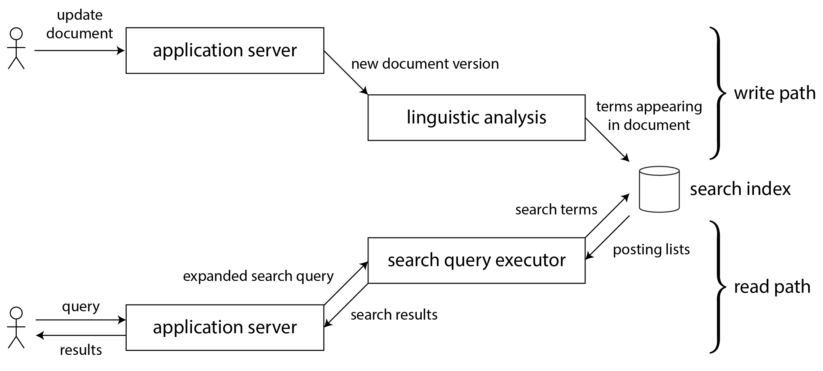
Figure 13-1 In a search index, writes (document updates) meet reads (queries).

But why do you create the derived dataset in the first place? Most likely because you want to query it again at a later time. This is the read path: when serving a user request you read from the derived dataset, perhaps perform some more processing on the results, and construct the response to the user.

Taken together, the write path and the read path encompass the whole journey of the data, from the point where it is collected to the point where it is consumed (probably by another human). The write path is the portion of the journey that is precomputed—i.e., that is done eagerly as soon as the data comes in, regardless of whether anyone has asked to see it. The read path is the portion of the journey that only happens when someone asks for it. If you are familiar with functional programming languages, you might notice that the write path is similar to eager evaluation, and the read path is similar to lazy evaluation.

The derived dataset is the place where the write path and the read path meet, as illustrated in Figure 13-1. It represents a trade-off between the amount of work that needs to be done at write time and the amount that needs to be done at read time.

Materialized views and caching

A full-text search index is a good example: the write path updates the index, and the read path searches the index for keywords. Both reads and writes need to do some work. Writes need to update the index entries for all terms that appear in the document. Reads need to search for each of the words in the query, and apply Boolean logic to find documents that contain all of the words in the query (an AND operator), or any synonym of each of the words (an OR operator).

If you didn’t have an index, a search query would have to scan over all documents (like grep), which would get very expensive if you had a large number of documents. No index means less work on the write path (no index to update), but a lot more work on the read path.

On the other hand, you could imagine precomputing the search results for all possible queries. In that case, you would have less work to do on the read path: no Boolean logic, just find the results for your query and return them. However, the write path would be a lot more expensive: the set of possible search queries that could be asked is infinite (or at least exponential in the number of terms in the corpus), and thus precomputing all possible search results would not be possible.

Another option would be to precompute the search results for only a fixed set of the most common queries, so that they can be served quickly without having to go to the index. The uncommon queries can still be served from the index. This would generally be called a cache of common queries, although we could also call it a materialized view, as it would need to be updated when new documents appear that should be included in the results of one of the common queries.

From this example we can see that an index is not the only possible boundary between the write path and the read path. Caching of common search results is possible, and grep-like scanning without the index is also possible on a small number of documents. Viewed like this, the role of caches, indexes, and materialized views is simple: they shift the boundary between the read path and the write path. They allow us to do more work on the write path, by precomputing results, in order to save effort on the read path.

Shifting the boundary between work done on the write path and the read path was in fact the topic of the social networking example in “Case Study: Social Network Home Timelines”. In that example, we also saw how the boundary between write path and read path might be drawn differently for celebrities compared to ordinary users. After 500 pages we have come full circle!

Stateful, offline-capable clients

The idea of a boundary between write and read paths is interesting because we can discuss shifting that boundary and explore what that shift means in practical terms. Let’s look at the idea in a different context.

In the past, web browsers were stateless clients that can only do useful things when you have an internet connection (just about the only thing you could do offline was to scroll up and down in a page that you had previously loaded while online). However, single-page JavaScript web apps now have a lot of stateful capabilities, including client-side user interface interaction and persistent local storage in the web browser. Mobile apps can similarly store a lot of state on the device and don’t require a round-trip to the server for most user interactions.

In “Sync Engines and Local-First Software” we saw how persistent local state enables a class of applications in which users can work offline, without an internet connection, and sync with remote servers in the background when a network connection is available ³⁰. Since mobile devices sometimes have slow and unreliable cellular internet connections, it’s a big advantage for users if their user interface does not have to wait for synchronous network requests, and if apps mostly work offline.

When we move away from the assumption of stateless clients talking to a central database and toward state that is maintained on end-user devices, a world of new opportunities opens up. In particular, we can think of the on-device state as a cache of state on the server. The pixels on the screen are a materialized view onto model objects in the client app; the model objects are a local replica of state in a remote datacenter ³¹.

Pushing state changes to clients

In a typical web page, if you load the page in a web browser and the data subsequently changes on the server, the browser does not find out about the change until you reload the page. The browser only reads the data at one point in time, assuming that it is static—it does not subscribe to updates from the server. Thus, the state in the browser is a stale cache that is not updated unless you explicitly poll for changes. (HTTP-based feed subscription protocols like RSS are really just a basic form of polling.)

More recent protocols have moved beyond the basic request/response pattern of HTTP: server-sent events (the EventSource API) and WebSockets provide communication channels by which a web browser can keep an open TCP connection to a server, and the server can actively push messages to the browser as long as it remains connected. This provides an opportunity for the server to actively inform the end-user client about any changes to the state it has stored locally, reducing the staleness of the client-side state.

In terms of our model of write path and read path, actively pushing state changes all the way to client devices means extending the write path all the way to the end user. When a client is first initialized, it would still need to use a read path to get its initial state, but thereafter it could rely on a stream of state changes sent by the server. The ideas we discussed around stream processing and messaging are not restricted to running only in a datacenter: we can take the ideas further, and extend them all the way to end-user devices ³².

The devices will be offline some of the time, and unable to receive any notifications of state changes from the server during that time. But we already solved that problem: in “Consumer offsets” we discussed how a consumer of a log-based message broker can reconnect after failing or becoming disconnected, and ensure that it doesn’t miss any messages that arrived while it was disconnected. The same technique works for individual users, where each device is a small subscriber to a small stream of events.

End-to-end event streams

Tools for developing stateful clients and user interfaces, such as React and Elm ³³, already have the ability to update the rendered user interface in response to changes in the underlying state. It would be very natural to extend this programming model to also allow a server to push state-change events into this client-side event pipeline.

Thus, state changes could flow through an end-to-end write path: from the interaction on one device that triggers a state change, via event logs and through several derived data systems and stream processors, all the way to the user interface of a person observing the state on another device. These state changes could be propagated with fairly low delay—say, under one second end to end.

Some applications, such as instant messaging and online games, already have such a “real-time” architecture (in the sense of interactions with low delay, not in the sense of response time guarantees). But why don’t we build all applications this way?

The challenge is that the assumption of stateless clients and request/response interactions is very deeply ingrained in our databases, libraries, frameworks, and protocols. Many datastores support read and write operations where a request returns one response, but much fewer provide an ability to subscribe to changes—i.e., a request that returns a stream of responses over time.

In order to extend the write path all the way to the end user, we would need to fundamentally rethink the way we build many of these systems: moving away from request/response interaction and toward publish/subscribe dataflow ³¹. This would require effort, but it would have the advantage of making user interfaces more responsive and providing better offline support.

Reads are events too

We discussed that when a stream processor writes derived data to a store (database, cache, or index), and that store is queried, the store acts as the boundary between the write path and the read path. The store allows random-access read queries to the data that would otherwise require scanning the whole event log.

In many cases, the data storage is separate from the streaming system. But recall that stream processors also need to maintain state to perform aggregations and joins. This state is normally hidden inside the stream processor, but some frameworks allow it to also be queried by outside clients ³⁴, turning the stream processor itself into a kind of simple database.

Let’s take that idea further. As discussed so far, the writes to the store go through an event log, while reads are transient network requests that go directly to the nodes that store the data being queried. This is a reasonable design, but not the only possible one. It is also possible to represent read requests as streams of events, and send both the read events and the write events through a stream processor; the processor responds to read events by emitting the result of the read to an output stream ³⁵.

When both the writes and the reads are represented as events, and routed to the same stream operator in order to be handled, we are in fact performing a stream-table join between the stream of read queries and the database. The read event needs to be sent to the database shard holding the data, just like batch and stream processors need to copartition inputs on the same key when joining.

This correspondence between serving requests and performing joins is quite fundamental ³⁶. A one-off read request passes through the join operator, which then immediately forgets the request; a subscribe request is a persistent join with past and future events on the other side of the join.

Recording a log of read events potentially also has benefits with regard to tracking causal dependencies and data provenance across a system: it would allow you to reconstruct what the user saw before they made a particular decision. For example, in an online shop, it is likely that the predicted shipping date and the inventory status shown to a customer affect whether they choose to buy an item ⁴. To analyze this connection, you need to record the result of the user’s query of the shipping and inventory status.

Writing read requests to durable storage thus enables better tracking of causal dependencies, but it incurs additional storage and I/O cost. Optimizing such systems to reduce the overhead is still an open research problem ². But if you already log read requests for operational purposes, as a side effect of request processing, it is not such a great change to make the log the source of the requests instead.

Multi-shard data processing

For queries that only touch a single shard, the effort of sending queries through a stream and collecting a stream of responses is perhaps overkill. However, this idea opens the possibility of distributed execution of complex queries that need to combine data from several shards, taking advantage of the infrastructure for message routing, sharding, and joining that is already provided by stream processors.

Storm’s distributed RPC feature supports this usage pattern. For example, it has been used to compute the number of people who have seen a URL on a social network—i.e., the union of the follower sets of everyone who has posted that URL ³⁷. As the set of users is sharded, this computation requires combining results from many shards.

Another example of this pattern occurs in fraud prevention: in order to assess the risk of whether a particular purchase event is fraudulent, you can examine the reputation scores of the user’s IP address, email address, billing address, shipping address, and so on. Each of these reputation databases is itself sharded, and so collecting the scores for a particular purchase event requires a sequence of joins with differently sharded datasets ³⁸.

The internal query execution graphs of data warehouse query engines have similar characteristics. If you need to perform this kind of multi-shard join, it is probably simpler to use a database that provides this feature than to implement it using a stream processor. However, treating queries as streams provides an option for implementing large-scale applications that run against the limits of conventional off-the-shelf solutions.

Aiming for Correctness

With stateless services that only read data, it is not a big deal if something goes wrong: you can fix the bug and restart the service, and everything returns to normal. Stateful systems such as databases are not so simple: they are designed to remember things forever (more or less), so if something goes wrong, the effects also potentially last forever—which means they require more careful thought ³⁹.

We want to build applications that are reliable and correct (i.e., programs whose semantics are well defined and understood, even in the face of various faults). For approximately four decades, the transaction properties of atomicity, isolation, and durability have been the tools of choice for building correct applications. However, those foundations are weaker than they seem: witness for example the confusion of weak isolation levels (see “Weak Isolation Levels”).

In some areas, transactions have been abandoned entirely and replaced with models that offer better performance and scalability, but much messier semantics. Consistency is often talked about, but poorly defined. Some people assert that we should “embrace weak consistency” for the sake of better availability, while lacking a clear idea of what that actually means in practice.

For a topic that is so important, our understanding and our engineering methods are surprisingly flaky. For example, it is very difficult to determine whether it is safe to run a particular application at a particular transaction isolation level or replication configuration ⁴⁰, ⁴¹. Often simple solutions appear to work correctly when concurrency is low and there are no faults, but turn out to have many subtle bugs in more demanding circumstances.

For example, Kyle Kingsbury’s Jepsen experiments ⁴² have highlighted the stark discrepancies between some products’ claimed safety guarantees and their actual behavior in the presence of network problems and crashes. Even if infrastructure products like databases were free from problems, application code would still need to correctly use the features they provide, which is error-prone if the configuration is hard to understand (which is the case with weak isolation levels, quorum configurations, and so on).

If your application can tolerate occasionally corrupting or losing data in unpredictable ways, life is a lot simpler, and you might be able to get away with simply crossing your fingers and hoping for the best. On the other hand, if you need stronger assurances of correctness, then serializability and atomic commit are established approaches, but they come at a cost: they typically only work in a single datacenter (ruling out geographically distributed architectures), and they limit the scale and fault-tolerance properties you can achieve.

While the traditional transaction approach is not going away, it is not the last word in making applications correct and resilient to faults. In this section we will explore some ways of thinking about correctness in the context of dataflow architectures.

The End-to-End Argument for Databases

Just because an application uses a data system that provides comparatively strong safety properties, such as serializable transactions, that does not mean the application is guaranteed to be free from data loss or corruption. For example, if an application has a bug that causes it to write incorrect data, or delete data from a database, serializable transactions aren’t going to save you. This is an argument in favor of immutable and append-only data, because it is easier to recover from such mistakes if you remove the ability of faulty code to destroy good data.

Although immutability is useful, it is not a cure-all by itself. Let’s look at a more subtle example of data corruption that can occur.

Exactly-once execution of an operation

In “Fault Tolerance” we encountered exactly-once (or effectively-once) semantics. If something goes wrong while processing a message, you can either give up (drop the message—i.e., incur data loss) or try again. If you try again, there is the risk that it actually succeeded the first time, but you just didn’t find out about the success, and so the message ends up being processed twice.

Processing twice is a form of data corruption: it is undesirable to charge a customer twice for the same service (billing them too much) or increment a counter twice (overstating some metric). In this context, exactly-once means arranging the computation such that the final effect is the same as if no faults had occurred, even if the operation actually was retried due to some fault. We previously discussed a few approaches for achieving this goal.

One of the most effective approaches is to make the operation idempotent; that is, to ensure that it has the same effect, no matter whether it is executed once or multiple times. However, taking an operation that is not naturally idempotent and making it idempotent requires some effort and care: you may need to maintain some additional metadata (such as the set of operation IDs that have updated a value), and ensure fencing when failing over from one node to another (see “Distributed Locks and Leases”).

Duplicate suppression

The same pattern of needing to suppress duplicates occurs in many other places besides stream processing. For example, TCP uses sequence numbers on packets to put them in the correct order at the recipient, and to determine whether any packets were lost or duplicated on the network. Any lost packets are retransmitted and any duplicates are removed by the TCP stack before it hands the data to an application.

However, this duplicate suppression only works within the context of a single TCP connection. Imagine the TCP connection is a client’s connection to a database, and it is currently executing the transaction in Example 13-1. In many databases, a transaction is tied to a client connection (if the client sends several queries, the database knows that they belong to the same transaction because they are sent on the same TCP connection). If the client suffers a network interruption and connection timeout after sending the COMMIT, but before hearing back from the database server, it does not know whether the transaction has been committed or aborted (Figure 9-1).

Example 13-1. A nonidempotent transfer of money from one account to another

BEGIN TRANSACTION;
UPDATE accounts SET balance = balance + 11.00 WHERE account_id = 1234;
UPDATE accounts SET balance = balance - 11.00 WHERE account_id = 4321;
COMMIT;

The client can reconnect to the database and retry the transaction, but now it is outside of the scope of TCP duplicate suppression. Since the transaction in Example 13-1 is not idempotent, it could happen that $22 is transferred instead of the desired $11. Thus, even though Example 13-1 is a standard example for transaction atomicity, it is actually not correct, and real banks do not work like this ³.

Two-phase commit (see “Two-Phase Commit (2PC)”) protocols break the 1:1 mapping between a TCP connection and a transaction, since they must allow a transaction coordinator to reconnect to a database after a network fault, and tell it whether to commit or abort an in-doubt transaction. Is this sufficient to ensure that the transaction will only be executed once? Unfortunately not.

Even if we can suppress duplicate transactions between the database client and server, we still need to worry about the network between the end-user device and the application server. For example, if the end-user client is a web browser, it probably uses an HTTP POST request to submit an instruction to the server. Perhaps the user is on a weak cellular data connection, and they succeed in sending the POST, but the signal becomes too weak before they are able to receive the response from the server.

In this case, the user will probably be shown an error message, and they may retry manually. Web browsers warn, “Are you sure you want to submit this form again?”—and the user says yes, because they wanted the operation to happen. (The Post/Redirect/Get pattern ⁴³ avoids this warning message in normal operation, but it doesn’t help if the POST request times out.) From the web server’s point of view the retry is a separate request, and from the database’s point of view it is a separate transaction. The usual deduplication mechanisms don’t help.

Uniquely identifying requests

To make the request idempotent through several hops of network communication, it is not sufficient to rely just on a transaction mechanism provided by a database—you need to consider the end-to-end flow of the request.

For example, you could generate a unique identifier for a request (such as a UUID) and include it as a hidden form field in the client application, or calculate a hash of all the relevant form fields to derive the request ID ³. If the web browser submits the POST request twice, the two requests will have the same request ID. You can then pass that request ID all the way through to the database and check that you only ever execute one request with a given ID, as shown in Example 13-2.

Example 13-2. Suppressing duplicate requests using a unique ID

ALTER TABLE requests ADD UNIQUE (request_id);

BEGIN TRANSACTION;

INSERT INTO requests
  (request_id, from_account, to_account, amount)
  VALUES('0286FDB8-D7E1-423F-B40B-792B3608036C', 4321, 1234, 11.00);

UPDATE accounts SET balance = balance + 11.00 WHERE account_id = 1234;
UPDATE accounts SET balance = balance - 11.00 WHERE account_id = 4321;

COMMIT;

Example 13-2 relies on a uniqueness constraint on the request_id column. If a transaction attempts to insert an ID that already exists, the INSERT fails and the transaction is aborted, preventing it from taking effect twice. Relational databases can generally maintain a uniqueness constraint correctly, even at weak isolation levels (whereas an application-level check-then-insert may fail under nonserializable isolation, as discussed in “Write Skew and Phantoms”).

Besides suppressing duplicate requests, the requests table in Example 13-2 acts as a kind of event log, which can be useful for event sourcing or change data capture. The updates to the account balances don’t actually have to happen in the same transaction as the insertion of the event, since they are redundant and could be derived from the request event in a downstream consumer—as long as the event is processed exactly once, which can again be enforced using the request ID.

The end-to-end argument

This scenario of suppressing duplicate transactions is just one example of a more general principle called the end-to-end argument, which was articulated by Saltzer, Reed, and Clark in 1984 ⁴⁴:

The function in question can completely and correctly be implemented only with the knowledge and help of the application standing at the endpoints of the communication system. Therefore, providing that questioned function as a feature of the communication system itself is not possible. (Sometimes an incomplete version of the function provided by the communication system may be useful as a performance enhancement.)

In our example, the function in question was duplicate suppression. We saw that TCP suppresses duplicate packets at the TCP connection level, and some stream processors provide so-called exactly-once semantics at the message processing level, but that is not enough to prevent a user from submitting a duplicate request if the first one times out. By themselves, TCP, database transactions, and stream processors cannot entirely rule out these duplicates. Solving the problem requires an end-to-end solution: a transaction identifier that is passed all the way from the end-user client to the database.

The end-to-end argument also applies to checking the integrity of data: checksums built into Ethernet, TCP, and TLS can detect corruption of packets in the network, but they cannot detect corruption due to bugs in the software at the sending and receiving ends of the network connection, or corruption on the disks where the data is stored. If you want to catch all possible sources of data corruption, you also need end-to-end checksums.

A similar argument applies with encryption ⁴⁴: the password on your home WiFi network protects against people snooping your WiFi traffic, but not against attackers elsewhere on the internet; TLS/SSL between your client and the server protects against network attackers, but not against compromises of the server. Only end-to-end encryption and authentication can protect against all of these things.

Although the low-level features (TCP duplicate suppression, Ethernet checksums, WiFi encryption) cannot provide the desired end-to-end features by themselves, they are still useful, since they reduce the probability of problems at the higher levels. For example, HTTP requests would often get mangled if we didn’t have TCP putting the packets back in the right order. We just need to remember that the low-level reliability features are not by themselves sufficient to ensure end-to-end correctness.

Applying end-to-end thinking in data systems

This brings us back to the original thesis: just because an application uses a data system that provides comparatively strong safety properties, such as serializable transactions, that does not mean the application is guaranteed to be free from data loss or corruption. The application itself needs to take end-to-end measures, such as duplicate suppression, as well.

That is a shame, because fault-tolerance mechanisms are hard to get right. Low-level reliability mechanisms, such as those in TCP, work quite well, and so the remaining higher-level faults occur fairly rarely. It would be really nice to wrap up the remaining high-level fault-tolerance machinery in an abstraction so that application code needn’t worry about it—but it seems that we have not yet found the right abstraction.

Transactions have long been seen as a useful abstraction. As discussed in Chapter 8, they take a wide range of possible issues (concurrent writes, constraint violations, crashes, network interruptions, disk failures) and collapse them down to two possible outcomes: commit or abort. That is a huge simplification of the programming model, but it is not enough.

Transactions are expensive, especially when they involve heterogeneous storage technologies (see “Distributed Transactions Across Different Systems”). When we refuse to use distributed transactions because they are too expensive, we end up having to reimplement fault-tolerance mechanisms in application code. As numerous examples throughout this book have shown, reasoning about concurrency and partial failure is difficult and counterintuitive, and so most application-level mechanisms do not work correctly. The consequence is lost or corrupted data.

For these reasons, it is worth exploring fault-tolerance abstractions that make it easy to provide application-specific end-to-end correctness properties, but also maintain good performance and good operational characteristics in a large-scale distributed environment.

Enforcing Constraints

Let’s think about correctness in the context of the ideas around unbundling databases. We saw that end-to-end duplicate suppression can be achieved with a request ID that is passed all the way from the client to the database that records the write. What about other kinds of constraints?

In particular, let’s focus on uniqueness constraints—such as the one we relied on in Example 13-2. In “Constraints and uniqueness guarantees” we saw several other examples of application features that need to enforce uniqueness: a username or email address must uniquely identify a user, a file storage service cannot have more than one file with the same name, and two people cannot book the same seat on a flight or in a theater.

Other kinds of constraints are very similar: for example, ensuring that an account balance never goes negative, that you don’t sell more items than you have in stock in the warehouse, or that a meeting room does not have overlapping bookings. Techniques that enforce uniqueness can often be used for these kinds of constraints as well.

Uniqueness constraints require consensus

In Chapter 10 we saw that in a distributed setting, enforcing a uniqueness constraint requires consensus: if there are several concurrent requests with the same value, the system somehow needs to decide which one of the conflicting operations is accepted, and reject the others as violations of the constraint.

The most common way of achieving this consensus is to make a single node the leader, and put it in charge of making all the decisions. That works fine as long as you don’t mind funneling all requests through a single node (even if the client is on the other side of the world), and as long as that node doesn’t fail. Consensus algorithms like Raft tackle the problem of safely electing a new leader if the current leader has failed (or is believed to have failed due to a network problem), and preventing split brain.

Uniqueness checking can be scaled out by sharding based on the value that needs to be unique. For example, if you need to ensure uniqueness by request ID, as in Example 13-2, you can ensure all requests with the same request ID are routed to the same shard. If you need usernames to be unique, you can shard by hash of username.

However, asynchronous multi-leader replication is ruled out, because it could happen that different leaders concurrently accept conflicting writes, and thus the values are no longer unique. If you want to be able to immediately reject any writes that would violate the constraint, synchronous coordination is unavoidable ⁴⁵.

Uniqueness in log-based messaging

A shared log ensures that all consumers see messages in the same order—a guarantee that is formally known as total order broadcast and is equivalent to consensus (see “The Many Faces of Consensus”). In the unbundled database approach with log-based messaging, we can use a very similar approach to enforce uniqueness constraints.

A stream processor consumes all the messages in a log shard sequentially on a single thread. Thus, if the log is sharded based on the value that needs to be unique, a stream processor can unambiguously and deterministically decide which one of several conflicting operations came first in the log. For example, in the case of several users trying to claim the same username ⁴⁶:

Every request for a username is encoded as a message, and appended to a shard determined by the hash of the username.
A stream processor sequentially reads the requests in the log, using a local database to keep track of which usernames are taken. For every request for a username that is available, it records the name as taken and emits a success message to an output stream. For every request for a username that is already taken, it emits a rejection message to an output stream.
The client that requested the username watches the output stream and waits for a success or rejection message corresponding to its request.

This algorithm is the same as the construction for achieving consensus using a shared log, which we saw in Chapter 10. It scales easily to a large request throughput by increasing the number of shards, as each shard can be processed independently.

The approach works not only for uniqueness constraints, but also for many other kinds of constraints. Its fundamental principle is that any writes that may conflict are routed to the same shard and processed sequentially. The definition of a conflict may depend on the application, but the stream processor can use arbitrary logic to validate a request.

Multi-shard request processing

Ensuring that an operation is executed atomically, while satisfying constraints, becomes more interesting when several shards are involved. In Example 13-2, there are potentially three shards: the one containing the request ID, the one containing the payee account, and the one containing the payer account. There is no reason why those three things should be in the same shard, since they are all independent from each other.

In the traditional approach to databases, executing this transaction would require an atomic commit across all three shards, which essentially forces it into a total order with respect to all other transactions on any of those shards. Since there is now cross-shard coordination, different shards can no longer be processed independently, so throughput is likely to suffer.

However, equivalent correctness can be achieved without cross-shard transactions using sharded logs and stream processors. Figure 13-2 shows an example of a payment transaction that needs to check whether there is sufficient money in the source account, and if so, atomically transfers some amount to a destination account while deducting fees. It works as follows ⁴⁷:

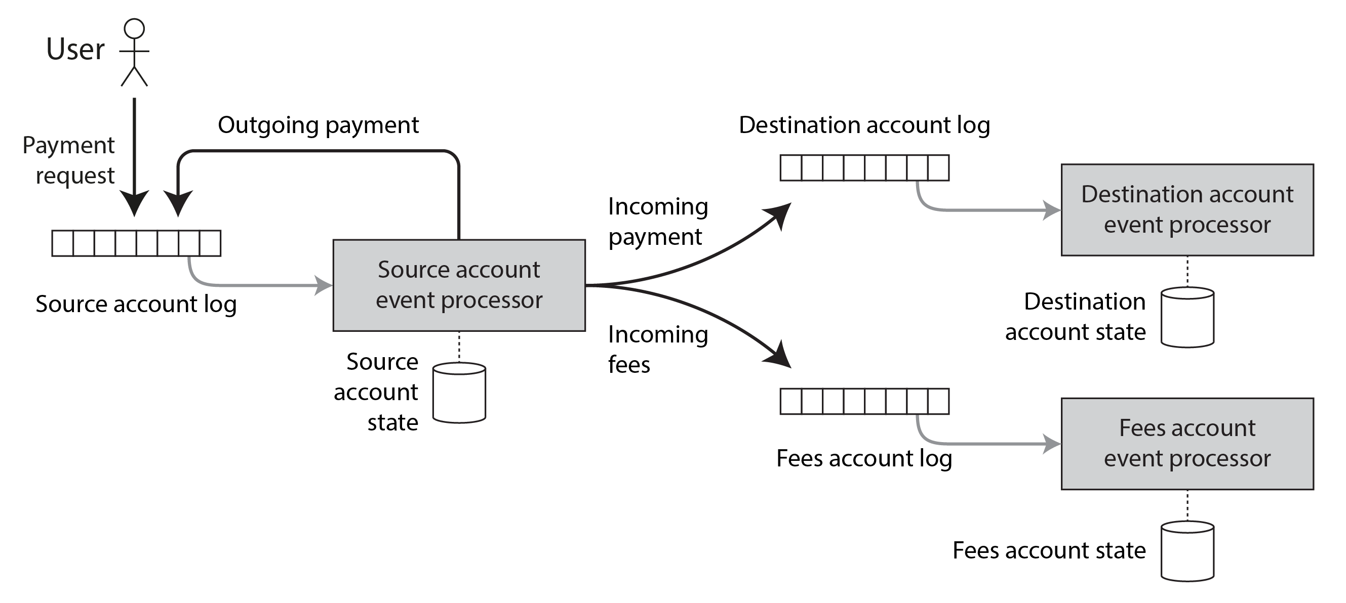
Figure 13-2 Checking whether a source account has enough money, and atomically transferring money to a destination account and a fees account, using event logs and stream processors.

The request to transfer money from the source account to the destination account is given a unique request ID by the user’s client, and appended to a log shard based on the source account ID.
A stream processor reads the log of requests and maintains a database containing the state of the source account and the IDs of requests it has already processed. The contents of this database are entirely derived from the log. When the stream processor encounters a request with an ID that it has not seen before, it checks in its local database whether the source account has enough money to perform the transfer.

If yes, it updates its local database to reserve the payment amount on the source account, and emits events to several other logs: an outgoing payment event to the log shard for the source account (its own input log), an incoming payment event to the log shard for the destination account, and an incoming payment event to the log shard for the fees account. The original request ID is included in those emitted events.
Eventually the outgoing payment event is delivered back to the source account processor (possibly after having received unrelated events in the meantime). The stream processor recognises based on the request ID that this is a payment it previously reserved, and it now executes the payment, again updating its local state of the source account. It ignores duplicates based on request ID.
The log shards for the destination and fees accounts are consumed by independent stream processing tasks. When they receive an incoming payment event, they update their local state to reflect the payment, and they deduplicate events based on request ID.

Figure 13-2 shows the three accounts as being in three separate shards, but they could just as well be in the same shards—it doesn’t matter. All we need is that the events for any given account are processed strictly in log order with at-least-once semantics, and that the stream processors are deterministic.

For example, consider what happens if the source account processor crashes while processing a payment request. The output messages may or may not have been emitted before the crash occurred. When it recovers from the crash, it will process the same request again (due to at-least-once semantics), and it will make the same decision on whether to allow the payment (since it’s deterministic). It will therefore emit the same output messages with the same request ID to the outgoing, incoming, and fees account shards. If they are duplicates, the downstream consumers will ignore them based on the request ID.

Atomicity in this system comes not from any transactions, but from the fact that writing the initial request event to the source account log is an atomic action. Once that one event in the log, all the downstream events will eventually be written as well—possibly after stream processors have recovered from crashes, and possibly with duplicates, but they will appear eventually.

With exactly-once semantics this example becomes easier to implement, since it ensures that the stream processor’s local state is consistent with the set of messages it has processed. Thus, if it crashes and re-processes some messages, its local state is also reset to what it was before those messages were processed.

If the user in Figure 13-2 wants to find out whether their transfer was approved or not, they can subscribe to the source account log shard and wait for the outgoing payment event. In order to explicitly notify the user if the balance is insufficient, the stream processor can emit a “declined payment” event to that log shard.

By breaking down the multi-shard transaction into several differently sharded stages and using the end-to-end request ID, we have achieved the same correctness property (every request is applied exactly once to both the payer and payee accounts), even in the presence of faults, and without using an atomic commit protocol.

Timeliness and Integrity

A convenient property of many transactional systems is that as soon as one transaction commits, its writes are immediately visible to other transactions. This property is formalized as strict serializability (see “Linearizability Versus Serializability”).

This is not the case when unbundling an operation across multiple stages of stream processors: consumers of a log are asynchronous by design, so a sender does not wait until its message has been processed by consumers. However, it is possible for a client to wait for a message to appear on an output stream, like the user waiting for an outgoing payment or payment declined event in Figure 13-2, which depends on whether there was enough money in the source account.

In this example, the correctness of the source account balance check does not depend on whether the user making the request waits for the outcome. The waiting only has the purpose of synchronously informing the user whether or not the payment succeeded, but this notification is decoupled from the effects of processing the request.

More generally, the term consistency conflates two different requirements that are worth considering separately:

Timeliness

Timeliness means ensuring that users observe the system in an up-to-date state. We saw previously that if a user reads from a stale copy of the data, they may observe it in an inconsistent state (see “Problems with Replication Lag”). However, that inconsistency is temporary, and will eventually be resolved simply by waiting and trying again.

The CAP theorem uses consistency in the sense of linearizability, which is a strong way of achieving timeliness. Weaker timeliness properties like read-after-write consistency can also be useful.

Integrity

Integrity means absence of corruption; i.e., no data loss, and no contradictory or false data. In particular, if some derived dataset is maintained as a view onto some underlying data, the derivation must be correct. For example, a database index must correctly reflect the contents of the database—an index in which some records are missing is not very useful.

If integrity is violated, the inconsistency is permanent: waiting and trying again is not going to fix database corruption in most cases. Instead, explicit checking and repair is needed. In the context of ACID transactions, “consistency” is usually understood as some kind of application-specific notion of integrity. Atomicity and durability are important tools for preserving integrity.

In slogan form: violations of timeliness are “eventual consistency,” whereas violations of integrity are “perpetual inconsistency.”

In most applications, integrity is much more important than timeliness. Violations of timeliness can be annoying and confusing, but violations of integrity can be catastrophic.

For example, on your credit card statement, it is not surprising if a transaction that you made within the last 24 hours does not yet appear—it is normal that these systems have a certain lag. We know that banks reconcile and settle transactions asynchronously, and timeliness is not very important here ³. However, it would be very bad if the statement balance was not equal to the sum of the transactions plus the previous statement balance (an error in the sums), or if a transaction was charged to you but not paid to the merchant (disappearing money). Such problems would be violations of the integrity of the system.

Correctness of dataflow systems

ACID transactions usually provide both timeliness (e.g., linearizability) and integrity (e.g., atomic commit) guarantees. Thus, if you approach application correctness from the point of view of ACID transactions, the distinction between timeliness and integrity is fairly inconsequential.

On the other hand, an interesting property of the event-based dataflow systems that we have discussed in this chapter is that they decouple timeliness and integrity. When processing event streams asynchronously, there is no guarantee of timeliness, unless you explicitly build consumers that wait for a message to arrive before returning. For example, a user could request a payment and then read the state of their account before the stream processor has executed the request; the user will not see the payment they just requested.

However, integrity is in fact central to streaming systems. Exactly-once or effectively-once semantics is a mechanism for preserving integrity. If an event is lost, or if an event takes effect twice, the integrity of a data system could be violated. Thus, fault-tolerant message delivery and duplicate suppression (e.g., idempotent operations) are important for maintaining the integrity of a data system in the face of faults.

As we saw in the last section, reliable stream processing systems can preserve integrity without requiring distributed transactions and an atomic commit protocol, which means they can potentially achieve comparable correctness with much better performance and operational robustness. We achieved this integrity through a combination of mechanisms:

Representing the content of the write operation as a single message, which can easily be written atomically—an approach that fits very well with event sourcing
Deriving all other state updates from that single message using deterministic derivation functions, similarly to stored procedures
Passing a client-generated request ID through all these levels of processing, enabling end-to-end duplicate suppression and idempotence
Making messages immutable and allowing derived data to be reprocessed from time to time, which makes it easier to recover from bugs

Loosely interpreted constraints

As discussed previously, enforcing a uniqueness constraint requires consensus, typically implemented by funneling all events in a particular shard through a single node. This limitation is unavoidable if we want the traditional form of uniqueness constraint, and stream processing cannot get around it.

However, another thing to realize is that in many real applications there is actually a business requirement to allow violations of what you might think of as hard constraints:

If customers order more items than you have in your warehouse, you can order in more stock, apologize to customers for the delay, and offer them a discount. This is actually the same as what you’d have to do if, say, a forklift truck ran over some of the items in your warehouse, leaving you with fewer items in stock than you thought you had ³. Thus, the apology workflow already needs to be part of your business processes anyway in order to deal with forklift incidents, and a hard constraint on the number of items in stock might be unnecessary.
Similarly, many airlines overbook airplanes in the expectation that some passengers will miss their flight, and many hotels overbook rooms, expecting that some guests will cancel. In these cases, the constraint of “one person per seat” is deliberately violated for business reasons, and compensation processes (refunds, upgrades, providing a complimentary room at a neighboring hotel) are put in place to handle situations in which demand exceeds supply. Even if there was no overbooking, apology and compensation processes would be needed in order to deal with flights being cancelled due to bad weather or staff on strike—recovering from such issues is just a normal part of business ³.
If someone withdraws more money than they have in their account, the bank can charge them an overdraft fee and ask them to pay back what they owe. By limiting the total withdrawals per day, the risk to the bank is bounded.
In systems that integrate data between different organizations, inconsistencies will inevitably arise, and correction mechanisms are necessary to handle them. As noted in “Batch Use Cases”, settlement of payments between banks is an example of this.

In many business contexts, it is therefore acceptable to temporarily violate a constraint and fix it up later by apologizing. This kind of change to correct a mistake is called a compensating transaction ⁴⁸, ⁴⁹. The cost of the apology (in terms of money or reputation) varies, but it is often quite low: you can’t unsend an email, but you can send a follow-up email with a correction. If you accidentally charge a credit card twice, you can refund one of the charges, and the cost to you is just the processing fees and perhaps a customer complaint. Once money has been paid out of an ATM, you can’t directly get it back, although in principle you can send debt collectors to recover the money if the account was overdrawn and the customer won’t pay it back.

Whether the cost of the apology is acceptable is a business decision. If it is acceptable, the traditional model of checking all constraints before even writing the data is unnecessarily restrictive. It may well be reasonable to go ahead with a write optimistically, and to check the constraint after the fact. You can still ensure that the validation occurs before doing things that would be expensive to recover from, but that doesn’t imply you must do the validation before you even write the data.

These applications do require integrity: you would not want to lose a reservation, or have money disappear due to mismatched credits and debits. But they don’t require timeliness on the enforcement of the constraint: if you have sold more items than you have in the warehouse, you can patch up the problem after the fact by apologizing. Doing so is similar to the conflict resolution approaches we discussed in “Dealing with Conflicting Writes”.

Coordination-avoiding data systems

We have now made two interesting observations:

Dataflow systems can maintain integrity guarantees on derived data without atomic commit, linearizability, or synchronous cross-shard coordination.
Although strict uniqueness constraints require timeliness and coordination, many applications are actually fine with loose constraints that may be temporarily violated and fixed up later, as long as integrity is preserved throughout.

Taken together, these observations mean that dataflow systems can provide the data management services for many applications without requiring coordination, while still giving strong integrity guarantees. Such coordination-avoiding data systems have a lot of appeal: they can achieve better performance and fault tolerance than systems that need to perform synchronous coordination ⁴⁵.

For example, such a system could operate distributed across multiple datacenters in a multi-leader configuration, asynchronously replicating between regions. Any one datacenter can continue operating independently from the others, because no synchronous cross-region coordination is required. Such a system would have weak timeliness guarantees—it could not be linearizable without introducing coordination—but it can still have strong integrity guarantees.

In this context, serializable transactions are still useful as part of maintaining derived state, but they can be run at a small scope where they work well ⁶. Heterogeneous distributed transactions such as XA transactions are not required. Synchronous coordination can still be introduced in places where it is needed (for example, to enforce strict constraints before an operation from which recovery is not possible), but there is no need for everything to pay the cost of coordination if only a small part of an application needs it ³².

Another way of looking at coordination and constraints: they reduce the number of apologies you have to make due to inconsistencies, but potentially also reduce the performance and availability of your system, and thus potentially increase the number of apologies you have to make due to outages. You cannot reduce the number of apologies to zero, but you can aim to find the best trade-off for your needs—the sweet spot where there are neither too many inconsistencies nor too many availability problems.

Trust, but Verify

All of our discussion of correctness, integrity, and fault-tolerance has been under the assumption that certain things might go wrong, but other things won’t. We call these assumptions our system model (see “System Model and Reality”): for example, we should assume that processes can crash, machines can suddenly lose power, and the network can arbitrarily delay or drop messages. But we might also assume that data written to disk is not lost after fsync, that data in memory is not corrupted, and that the multiplication instruction of our CPU always returns the correct result.

These assumptions are quite reasonable, as they are true most of the time, and it would be difficult to get anything done if we had to constantly worry about our computers making mistakes. Traditionally, system models take a binary approach toward faults: we assume that some things can happen, and other things can never happen. In reality, it is more a question of probabilities: some things are more likely, other things less likely. The question is whether violations of our assumptions happen often enough that we may encounter them in practice.

We have seen that data can become corrupted in memory (see “Hardware and Software Faults”), on disk (see “Replication and Durability”), and on the network (see “Weak forms of lying”). Maybe this is something we should be paying more attention to? If you are operating at large enough scale, even very unlikely things do happen.

Maintaining integrity in the face of software bugs

Besides such hardware issues, there is always the risk of software bugs, which would not be caught by lower-level network, memory, or filesystem checksums. Even widely used database software has bugs: for example, past versions of MySQL have failed to correctly maintain uniqueness constraints ⁵⁰ and PostgreSQL’s serializable isolation level has exhibited write skew anomalies in the past ⁵¹, even though MySQL and PostgreSQL are robust and well-regarded databases that have been battle-tested by many people for many years. In less mature software, the situation is likely to be much worse.

Despite considerable efforts in careful design, testing, and review, bugs still creep in. Although they are rare, and they eventually get found and fixed, there is still a period during which such bugs can corrupt data.

When it comes to application code, we have to assume many more bugs, since most applications don’t receive anywhere near the amount of review and testing that database code does. Many applications don’t even correctly use the features that databases offer for preserving integrity, such as foreign key or uniqueness constraints ²⁵.

Consistency in the sense of ACID is based on the idea that the database starts off in a consistent state, and a transaction transforms it from one consistent state to another consistent state. Thus, we expect the database to always be in a consistent state. However, this notion only makes sense if you assume that the transaction is free from bugs. If the application uses the database incorrectly in some way, for example using a weak isolation level unsafely, the integrity of the database cannot be guaranteed.

Don’t just blindly trust what they promise

With both hardware and software not always living up to the ideal that we would like them to be, it seems that data corruption is inevitable sooner or later. Thus, we should at least have a way of finding out if data has been corrupted so that we can fix it and try to track down the source of the error. Checking the integrity of data is known as auditing.

As discussed in “Advantages of immutable events”, auditing is not just for financial applications. However, auditability is very important in finance precisely because everyone knows that mistakes happen, and we all recognize the need to be able to detect and fix problems.

Mature systems similarly tend to consider the possibility of unlikely things going wrong, and manage that risk. For example, large-scale storage systems such as HDFS and Amazon S3 do not fully trust disks: they run background processes that continually read back files, compare them to other replicas, and move files from one disk to another, in order to mitigate the risk of silent corruption ⁵², ⁵³.

If you want to be sure that your data is still there, you have to actually read it and check. Most of the time it will still be there, but if it isn’t, you really want to find out sooner rather than later. By the same argument, it is important to try restoring from your backups from time to time—otherwise you may only find out that your backup is broken when it is too late and you have already lost data. Don’t just blindly trust that it is all working.

Systems like HDFS and S3 still have to assume that disks work correctly most of the time—which is a reasonable assumption, but not the same as assuming that they always work correctly. However, not many systems currently have this kind of “trust, but verify” approach of continually auditing themselves. Many assume that correctness guarantees are absolute and make no provision for the possibility of rare data corruption. In the future we may see more self-validating or self-auditing systems that continually check their own integrity, rather than relying on blind trust ⁵⁴.

Designing for auditability

If a transaction mutates several objects in a database, it is difficult to tell after the fact what that transaction means. Even if you capture the transaction logs, the insertions, updates, and deletions in various tables do not necessarily give a clear picture of why those mutations were performed. The invocation of the application logic that decided on those mutations is transient and cannot be reproduced.

By contrast, event-based systems can provide better auditability. In the event sourcing approach, user input to the system is represented as a single immutable event, and any resulting state updates are derived from that event. The derivation can be made deterministic and repeatable, so that running the same log of events through the same version of the derivation code will result in the same state updates.

Being explicit about dataflow makes the provenance of data much clearer, which makes integrity checking much more feasible. For the event log, we can use hashes to check that the event storage has not been corrupted. For any derived state, we can rerun the batch and stream processors that derived it from the event log in order to check whether we get the same result, or even run a redundant derivation in parallel.

A deterministic and well-defined dataflow also makes it easier to debug and trace the execution of a system in order to determine why it did something ⁴, ⁵⁵. If something unexpected occurred, it is valuable to have the diagnostic capability to reproduce the exact circumstances that led to the unexpected event—a kind of time-travel debugging capability.

The end-to-end argument again

If we cannot fully trust that every individual component of the system will be free from corruption—that every piece of hardware is fault-free and that every piece of software is bug-free—then we must at least periodically check the integrity of our data. If we don’t check, we won’t find out about corruption until it is too late and it has caused some downstream damage, at which point it will be much harder and more expensive to track down the problem.

Checking the integrity of data systems is best done in an end-to-end fashion: the more systems we can include in an integrity check, the fewer opportunities there are for corruption to go unnoticed at some stage of the process. If we can check that an entire derived data pipeline is correct end to end, then any disks, networks, services, and algorithms along the path are implicitly included in the check.

Having continuous end-to-end integrity checks gives you increased confidence about the correctness of your systems, which in turn allows you to move faster ⁵⁶. Like automated testing, auditing increases the chances that bugs will be found quickly, and thus reduces the risk that a change to the system or a new storage technology will cause damage. If you are not afraid of making changes, you can much better evolve an application to meet changing requirements.

Tools for auditable data systems

At present, not many data systems make auditability a top-level concern. Some applications implement their own audit mechanisms, for example by logging all changes to a separate audit table, but guaranteeing the integrity of the audit log and the database state is still difficult. A transaction log can be made tamper-proof by periodically signing it with a hardware security module, but that does not guarantee that the right transactions went into the log in the first place.

Blockchains such as Bitcoin or Ethereum are shared append-only logs with cryptographic consistency checks; the transactions they store are events, and smart contracts are basically stream processors. The consensus protocols they use ensure that all nodes agree on the same sequence of events. The difference to the consensus protocols of Chapter 10 is that blockchains are Byzantine fault tolerant, i.e. they still work if some of the participating nodes have corrupted data because the replicas continually check each other’s integrity.

For most applications, blockchains have too high overhead to be useful. However, some of their cryptographic tools can also be used in a lighterweight context. For example, Merkle trees ⁵⁷, are trees of hashes that can be used to efficiently prove that a record appears in some dataset (and a few other things). Certificate transparency uses cryptographically verified append-only logs and Merkle trees to check the validity of TLS/SSL certificates ⁵⁸, ⁵⁹; it avoids needing a consensus protocol by having a single leader per log.

Integrity-checking and auditing algorithms, like those of certificate transparency and distributed ledgers, might becoming more widely used in data systems in general in the future. Some work will be needed to make them equally scalable as systems without cryptographic auditing, and to keep the performance penalty as low as possible, but they are nevertheless interesting.

Summary

In this chapter we discussed new approaches to designing data systems based on ideas from stream processing. We started with the observation that there is no one single tool that can efficiently serve all possible use cases, and so applications necessarily need to compose several different pieces of software to accomplish their goals. We discussed how to solve this data integration problem by using batch processing and event streams to let data changes flow between different systems.

In this approach, certain systems are designated as systems of record, and other data is derived from them through transformations. In this way we can maintain indexes, materialized views, machine learning models, statistical summaries, and more. By making these derivations and transformations asynchronous and loosely coupled, a problem in one area is prevented from spreading to unrelated parts of the system, increasing the robustness and fault-tolerance of the system as a whole.

Expressing dataflows as transformations from one dataset to another also helps evolve applications: if you want to change one of the processing steps, for example to change the structure of an index or cache, you can just rerun the new transformation code on the whole input dataset in order to rederive the output. Similarly, if something goes wrong, you can fix the code and reprocess the data in order to recover.

These processes are quite similar to what databases already do internally, so we recast the idea of dataflow applications as unbundling the components of a database, and building an application by composing these loosely coupled components.

Derived state can be updated by observing changes in the underlying data. Moreover, the derived state itself can further be observed by downstream consumers. We can even take this dataflow all the way through to the end-user device that is displaying the data, and thus build user interfaces that dynamically update to reflect data changes and continue to work offline.

Next, we discussed how to ensure that all of this processing remains correct in the presence of faults. We saw that strong integrity guarantees can be implemented scalably with asynchronous event processing, by using end-to-end request identifiers to make operations idempotent and by checking constraints asynchronously. Clients can either wait until the check has passed, or go ahead without waiting but risk having to apologize about a constraint violation. This approach is much more scalable and robust than the traditional approach of using distributed transactions, and fits with how many business processes work in practice.

By structuring applications around dataflow and checking constraints asynchronously, we can avoid most coordination and create systems that maintain integrity but still perform well, even in geographically distributed scenarios and in the presence of faults. We then talked a little about using audits to verify the integrity of data and detect corruption, and observed that the techniques used by blockchains also have a similarity to event-based systems.

Footnotes

References

Rachid Belaid. Postgres Full-Text Search is Good Enough! rachbelaid.com, July 2015. Archived at perma.cc/ZVP9-YDCB ↩︎ ↩︎
Philippe Ajoux, Nathan Bronson, Sanjeev Kumar, Wyatt Lloyd, and Kaushik Veeraraghavan. Challenges to Adopting Stronger Consistency at Scale. At 15th USENIX Workshop on Hot Topics in Operating Systems (HotOS), May 2015. ↩︎ ↩︎
Pat Helland and Dave Campbell. Building on Quicksand. At 4th Biennial Conference on Innovative Data Systems Research (CIDR), January 2009. ↩︎ ↩︎ ↩︎ ↩︎ ↩︎ ↩︎
Jessica Kerr. Provenance and Causality in Distributed Systems. jessitron.com, September 2016. Archived at perma.cc/DTD2-F8ZM ↩︎ ↩︎ ↩︎
Jay Kreps. The Log: What Every Software Engineer Should Know About Real-Time Data’s Unifying Abstraction. engineering.linkedin.com, December 2013. Archived at perma.cc/2JHR-FR64 ↩︎ ↩︎ ↩︎ ↩︎
Pat Helland. Life Beyond Distributed Transactions: An Apostate’s Opinion. At 3rd Biennial Conference on Innovative Data Systems Research (CIDR), January 2007. ↩︎ ↩︎
Lionel A. Smith. The Broad Gauge Story. Journal of the Monmouthshire Railway Society, Summer 1985. Archived at perma.cc/DDK9-JA6X ↩︎
Jacqueline Xu. Online Migrations at Scale. stripe.com, February 2017. Archived at perma.cc/ZQY2-EAU2 ↩︎
Flavio Santos and Robert Stephenson. Changing the Wheels on a Moving Bus — Spotify’s Event Delivery Migration. engineering.atspotify.com, October 2021. Archived at perma.cc/5C4V-G8EV ↩︎
Molly Bartlett Dishman and Martin Fowler. Agile Architecture. At O’Reilly Software Architecture Conference, March 2015. ↩︎
Nathan Marz and James Warren. Big Data: Principles and Best Practices of Scalable Real-Time Data Systems. Manning, 2015. ISBN: 978-1-617-29034-3 ↩︎
Jay Kreps. Questioning the Lambda Architecture. oreilly.com, July 2014. Archived at perma.cc/PGH6-XUCH ↩︎ ↩︎
Raul Castro Fernandez, Peter Pietzuch, Jay Kreps, Neha Narkhede, Jun Rao, Joel Koshy, Dong Lin, Chris Riccomini, and Guozhang Wang. Liquid: Unifying Nearline and Offline Big Data Integration. At 7th Biennial Conference on Innovative Data Systems Research (CIDR), January 2015. ↩︎
Dennis M. Ritchie and Ken Thompson. The UNIX Time-Sharing System. Communications of the ACM, volume 17, issue 7, pages 365–375, July 1974. doi:10.1145/361011.361061 ↩︎ ↩︎
Wes McKinney. The Road to Composable Data Systems: Thoughts on the Last 15 Years and the Future. wesmckinney.com, September 2023. Archived at perma.cc/J9SJ-886N ↩︎
Eric A. Brewer and Joseph M. Hellerstein. CS262a: Advanced Topics in Computer Systems. Lecture notes, University of California, Berkeley, cs.berkeley.edu, August 2011. Archived at perma.cc/TE79-LGWU ↩︎
Michael Stonebraker. The Case for Polystores. wp.sigmod.org, July 2015. Archived at perma.cc/G7J2-KR45 ↩︎ ↩︎
Jennie Duggan, Aaron J. Elmore, Michael Stonebraker, Magda Balazinska, Bill Howe, Jeremy Kepner, Sam Madden, David Maier, Tim Mattson, and Stan Zdonik. The BigDAWG Polystore System. ACM SIGMOD Record, volume 44, issue 2, pages 11–16, June 2015. doi:10.1145/2814710.2814713 ↩︎
David B. Lomet, Alan Fekete, Gerhard Weikum, and Mike Zwilling. Unbundling Transaction Services in the Cloud. At 4th Biennial Conference on Innovative Data Systems Research (CIDR), January 2009. ↩︎
Martin Kleppmann and Jay Kreps. Kafka, Samza and the Unix Philosophy of Distributed Data. IEEE Data Engineering Bulletin, volume 38, issue 4, pages 4–14, December 2015. ↩︎
John Hugg. Winning Now and in the Future: Where Volt Active Data Shines. voltactivedata.com, March 2016. Archived at perma.cc/44MP-3MWM ↩︎
Felienne Hermans. Spreadsheets Are Code. At Code Mesh, November 2015. ↩︎
Dan Bricklin and Bob Frankston. VisiCalc: Information from Its Creators. danbricklin.com. Archived at archive.org ↩︎
D. Sculley, Gary Holt, Daniel Golovin, Eugene Davydov, Todd Phillips, Dietmar Ebner, Vinay Chaudhary, and Michael Young. Machine Learning: The High-Interest Credit Card of Technical Debt. At NIPS Workshop on Software Engineering for Machine Learning (SE4ML), December 2014. Archived at https://perma.cc/M3MD-U7WL ↩︎
Peter Bailis, Alan Fekete, Michael J. Franklin, Ali Ghodsi, Joseph M. Hellerstein, and Ion Stoica. Feral Concurrency Control: An Empirical Investigation of Modern Application Integrity. At ACM International Conference on Management of Data (SIGMOD), June 2015. doi:10.1145/2723372.2737784 ↩︎ ↩︎
Guy Steele. Re: Need for Macros (Was Re: Icon). email to ll1-discuss mailing list, people.csail.mit.edu, December 2001. Archived at perma.cc/K9X8-CJ65 ↩︎
Ben Stopford. Microservices in a Streaming World. At QCon London, March 2016. ↩︎ ↩︎
Adam Bellemare. Building Event-Driven Microservices, 2nd Edition. O’Reilly Media, 2025. ↩︎
Christian Posta. Why Microservices Should Be Event Driven: Autonomy vs Authority. blog.christianposta.com, May 2016. Archived at perma.cc/E6N9-3X92 ↩︎
Alex Feyerke. Designing Offline-First Web Apps. alistapart.com, December 2013. Archived at perma.cc/WH7R-S2DS ↩︎
Martin Kleppmann. Turning the Database Inside-out with Apache Samza. at Strange Loop, September 2014. Archived at perma.cc/U6E8-A9MT ↩︎ ↩︎
Sebastian Burckhardt, Daan Leijen, Jonathan Protzenko, and Manuel Fähndrich. Global Sequence Protocol: A Robust Abstraction for Replicated Shared State. At 29th European Conference on Object-Oriented Programming (ECOOP), July 2015. doi:10.4230/LIPIcs.ECOOP.2015.568 ↩︎ ↩︎
Evan Czaplicki and Stephen Chong. Asynchronous Functional Reactive Programming for GUIs. At 34th ACM SIGPLAN Conference on Programming Language Design and Implementation (PLDI), June 2013. doi:10.1145/2491956.2462161 ↩︎
Eno Thereska, Damian Guy, Michael Noll, and Neha Narkhede. Unifying Stream Processing and Interactive Queries in Apache Kafka. confluent.io, October 2016. Archived at perma.cc/W8JG-EAZF ↩︎
Frank McSherry. Dataflow as Database. github.com, July 2016. Archived at perma.cc/384D-DUFH ↩︎
Peter Alvaro. I See What You Mean. At Strange Loop, September 2015. ↩︎
Nathan Marz. Trident: A High-Level Abstraction for Realtime Computation. blog.x.com, August 2012. Archived at archive.org ↩︎
Edi Bice. Low Latency Web Scale Fraud Prevention with Apache Samza, Kafka and Friends. At Merchant Risk Council MRC Vegas Conference, March 2016. Archived at perma.cc/T3H5-QN3R ↩︎
Charity Majors. The Accidental DBA. charity.wtf, October 2016. Archived at perma.cc/6ANP-ARB6 ↩︎
Arthur J. Bernstein, Philip M. Lewis, and Shiyong Lu. Semantic Conditions for Correctness at Different Isolation Levels. At 16th International Conference on Data Engineering (ICDE), February 2000. doi:10.1109/ICDE.2000.839387 ↩︎
Sudhir Jorwekar, Alan Fekete, Krithi Ramamritham, and S. Sudarshan. Automating the Detection of Snapshot Isolation Anomalies. At 33rd International Conference on Very Large Data Bases (VLDB), September 2007. ↩︎
Kyle Kingsbury. Jepsen: Distributed Systems Safety Research. jepsen.io. ↩︎
Michael Jouravlev. Redirect After Post. theserverside.com, August 2004. Archived at archive.org ↩︎
Jerome H. Saltzer, David P. Reed, and David D. Clark. End-to-End Arguments in System Design. ACM Transactions on Computer Systems, volume 2, issue 4, pages 277–288, November 1984. doi:10.1145/357401.357402 ↩︎ ↩︎
Peter Bailis, Alan Fekete, Michael J. Franklin, Ali Ghodsi, Joseph M. Hellerstein, and Ion Stoica. Coordination Avoidance in Database Systems. Proceedings of the VLDB Endowment, volume 8, issue 3, pages 185–196, November 2014. doi:10.14778/2735508.2735509 ↩︎ ↩︎
Alex Yarmula. Strong Consistency in Manhattan. blog.x.com, March 2016. Archived at archive.org ↩︎
Martin Kleppmann, Alastair R. Beresford, and Boerge Svingen. Online Event Processing: Achieving consistency where distributed transactions have failed. Communications of the ACM, volume 62, issue 5, pages 43-49, May 2019. doi:10.1145/3312527 ↩︎
Jim Gray. The Transaction Concept: Virtues and Limitations. At 7th International Conference on Very Large Data Bases (VLDB), September 1981. Archived at perma.cc/8VPT-N5H6 ↩︎
Hector Garcia-Molina and Kenneth Salem. Sagas. At ACM International Conference on Management of Data (SIGMOD), May 1987. doi:10.1145/38713.38742 ↩︎
Annamalai Gurusami and Daniel Price. Bug #73170: Duplicates in Unique Secondary Index Because of Fix of Bug#68021. bugs.mysql.com, July 2014. Archived at perma.cc/P6BV-W7JJ ↩︎
Gary Fredericks. Postgres Serializability Bug. github.com, September 2015. Archived at perma.cc/N8UP-2822 ↩︎
Xiao Chen. HDFS DataNode Scanners and Disk Checker Explained. blog.cloudera.com, December 2016. Archived at perma.cc/6S36-X98L ↩︎
Daniel Persson. How does Ceph scrubbing work? youtube.com, March 2022. ↩︎
Jay Kreps. Getting Real About Distributed System Reliability. blog.empathybox.com, March 2012. Archived at perma.cc/9B5Q-AEBW ↩︎
Martin Fowler. The LMAX Architecture. martinfowler.com, July 2011. Archived at perma.cc/5AV4-N6RJ ↩︎
Sam Stokes. Move Fast with Confidence. five-eights.com, July 2016. Archived at perma.cc/J8C6-DHXB ↩︎
Ralph C. Merkle. A Digital Signature Based on a Conventional Encryption Function. At CRYPTO ‘87, August 1987. doi:10.1007/3-540-48184-2_32 ↩︎
Ben Laurie. Certificate Transparency. ACM Queue, volume 12, issue 8, pages 10-19, August 2014. doi:10.1145/2668152.2668154 ↩︎
Mark D. Ryan. Enhanced Certificate Transparency and End-to-End Encrypted Mail. At Network and Distributed System Security Symposium (NDSS), February 2014. doi:10.14722/ndss.2014.23379 ↩︎

14. Doing the Right Thing

Feeding AI systems on the world’s beauty, ugliness, and cruelty, but expecting it to reflect only the beauty is a fantasy.

Vinay Uday Prabhu and Abeba Birhane, Large Datasets: A Pyrrhic Win for Computer Vision? (2020)

A NOTE FOR EARLY RELEASE READERS

This will be the 14th chapter of the final book. The GitHub repo for this book is https://github.com/ept/ddia2-feedback.

If you’d like to be actively involved in reviewing and commenting on this draft, please reach out on GitHub.

In the final chapter of this book, let’s take a step back. Throughout this book we have examined a wide range of different architectures for data systems, evaluated their pros and cons, and explored techniques for building reliable, scalable, and maintainable applications. However, we have left out an important and fundamental part of the discussion, which we should now fill in.

Every system is built for a purpose; every action we take has both intended and unintended consequences. The purpose may be as simple as making money, but the consequences for the world may reach far beyond that original purpose. We, the engineers building these systems, have a responsibility to carefully consider those consequences and to consciously decide what kind of world we want to live in.

We talk about data as an abstract thing, but remember that many datasets are about people: their behavior, their interests, their identity. We must treat such data with humanity and respect. Users are humans too, and human dignity is paramount ¹.

Software development increasingly involves making important ethical choices. There are guidelines to help software engineers navigate these issues, such as the ACM Code of Ethics and Professional Conduct ², but they are rarely discussed, applied, and enforced in practice. As a result, engineers and product managers sometimes take a very cavalier attitude to privacy and potential negative consequences of their products ³, ⁴.

A technology is not good or bad in itself—what matters is how it is used and how it affects people. This is true for a software system like a search engine in much the same way as it is for a weapon like a gun. Is not sufficient for software engineers to focus exclusively on the technology and ignore its consequences: the ethical responsibility is ours to bear also. Reasoning about ethics is difficult, but it is too important to ignore.

However, what makes something “good” or “bad” is not well-defined, and most people in computing don’t even discuss that question ⁵. In contrast to much of computing, the concepts at the heart of ethics are not fixed or determinate in their precise meaning, and they require interpretation, which may be subjective ⁶. Ethics is not going through some checklist to confirm you comply; it’s a participatory and iterative process of reflection, in dialog with the people involved, with accountability for the results ⁷.

Predictive Analytics

For example, predictive analytics is a major part of why people are excited about big data and AI. Using data analysis to predict the weather, or the spread of diseases, is one thing ⁸; it is another matter to predict whether a convict is likely to reoffend, whether an applicant for a loan is likely to default, or whether an insurance customer is likely to make expensive claims ⁹. The latter have a direct effect on individual people’s lives.

Naturally, payment networks want to prevent fraudulent transactions, banks want to avoid bad loans, airlines want to avoid hijackings, and companies want to avoid hiring ineffective or untrustworthy people. From their point of view, the cost of a missed business opportunity is low, but the cost of a bad loan or a problematic employee is much higher, so it is natural for organizations to want to be cautious. If in doubt, they are better off saying no.

However, as algorithmic decision-making becomes more widespread, someone who has (accurately or falsely) been labeled as risky by some algorithm may suffer a large number of those “no” decisions. Systematically being excluded from jobs, air travel, insurance coverage, property rental, financial services, and other key aspects of society is such a large constraint of the individual’s freedom that it has been called “algorithmic prison” ¹⁰. In countries that respect human rights, the criminal justice system presumes innocence until proven guilty; on the other hand, automated systems can systematically and arbitrarily exclude a person from participating in society without any proof of guilt, and with little chance of appeal.

Bias and Discrimination

Decisions made by an algorithm are not necessarily any better or any worse than those made by a human. Every person is likely to have biases, even if they actively try to counteract them, and discriminatory practices can become culturally institutionalized. There is hope that basing decisions on data, rather than subjective and instinctive assessments by people, could be more fair and give a better chance to people who are often overlooked in the traditional system ¹¹.

When we develop predictive analytics and AI systems, we are not merely automating a human’s decision by using software to specify the rules for when to say yes or no; we are even leaving the rules themselves to be inferred from data. However, the patterns learned by these systems are opaque: even if there is some correlation in the data, we may not know why. If there is a systematic bias in the input to an algorithm, the system will most likely learn and amplify that bias in its output ¹².

In many countries, anti-discrimination laws prohibit treating people differently depending on protected traits such as ethnicity, age, gender, sexuality, disability, or beliefs. Other features of a person’s data may be analyzed, but what happens if they are correlated with protected traits? For example, in racially segregated neighborhoods, a person’s postal code or even their IP address is a strong predictor of race. Put like this, it seems ridiculous to believe that an algorithm could somehow take biased data as input and produce fair and impartial output from it ¹³, ¹⁴. Yet this belief often seems to be implied by proponents of data-driven decision making, an attitude that has been satirized as “machine learning is like money laundering for bias” ¹⁵.

Predictive analytics systems merely extrapolate from the past; if the past is discriminatory, they codify and amplify that discrimination ¹⁶. If we want the future to be better than the past, moral imagination is required, and that’s something only humans can provide ¹⁷. Data and models should be our tools, not our masters.

Responsibility and Accountability

Automated decision making opens the question of responsibility and accountability ¹⁷. If a human makes a mistake, they can be held accountable, and the person affected by the decision can appeal. Algorithms make mistakes too, but who is accountable if they go wrong ¹⁸? When a self-driving car causes an accident, who is responsible? If an automated credit scoring algorithm systematically discriminates against people of a particular race or religion, is there any recourse? If a decision by your machine learning system comes under judicial review, can you explain to the judge how the algorithm made its decision? People should not be able to evade their responsibility by blaming an algorithm.

Credit rating agencies are an old example of collecting data to make decisions about people. A bad credit score makes life difficult, but at least a credit score is normally based on relevant facts about a person’s actual borrowing history, and any errors in the record can be corrected (although the agencies normally do not make this easy). However, scoring algorithms based on machine learning typically use a much wider range of inputs and are much more opaque, making it harder to understand how a particular decision has come about and whether someone is being treated in an unfair or discriminatory way ¹⁹.

A credit score summarizes “How did you behave in the past?” whereas predictive analytics usually work on the basis of “Who is similar to you, and how did people like you behave in the past?” Drawing parallels to others’ behavior implies stereotyping people, for example based on where they live (a close proxy for race and socioeconomic class). What about people who get put in the wrong bucket? Furthermore, if a decision is incorrect due to erroneous data, recourse is almost impossible ¹⁷.

Much data is statistical in nature, which means that even if the probability distribution on the whole is correct, individual cases may well be wrong. For example, if the average life expectancy in your country is 80 years, that doesn’t mean you’re expected to drop dead on your 80th birthday. From the average and the probability distribution, you can’t say much about the age to which one particular person will live. Similarly, the output of a prediction system is probabilistic and may well be wrong in individual cases.

A blind belief in the supremacy of data for making decisions is not only delusional, it is positively dangerous. As data-driven decision making becomes more widespread, we will need to figure out how to make algorithms accountable and transparent, how to avoid reinforcing existing biases, and how to fix them when they inevitably make mistakes.

We will also need to figure out how to prevent data being used to harm people, and realize its positive potential instead. For example, analytics can reveal financial and social characteristics of people’s lives. On the one hand, this power could be used to focus aid and support to help those people who most need it. On the other hand, it is sometimes used by predatory business seeking to identify vulnerable people and sell them risky products such as high-cost loans and worthless college degrees ¹⁷, ²⁰.

Feedback Loops

Even with predictive applications that have less immediately far-reaching effects on people, such as recommendation systems, there are difficult issues that we must confront. When services become good at predicting what content users want to see, they may end up showing people only opinions they already agree with, leading to echo chambers in which stereotypes, misinformation, and polarization can breed. We are already seeing the impact of social media echo chambers on election campaigns.

When predictive analytics affect people’s lives, particularly pernicious problems arise due to self-reinforcing feedback loops. For example, consider the case of employers using credit scores to evaluate potential hires. You may be a good worker with a good credit score, but suddenly find yourself in financial difficulties due to a misfortune outside of your control. As you miss payments on your bills, your credit score suffers, and you will be less likely to find work. Joblessness pushes you toward poverty, which further worsens your scores, making it even harder to find employment ¹⁷. It’s a downward spiral due to poisonous assumptions, hidden behind a camouflage of mathematical rigor and data.

As another example of a feedback loop, economists found that when gas stations in Germany introduced algorithmic prices, competition was reduced and prices for consumers went up because the algorithms learned to collude ²¹.

We can’t always predict when such feedback loops happen. However, many consequences can be predicted by thinking about the entire system (not just the computerized parts, but also the people interacting with it)—an approach known as systems thinking ²². We can try to understand how a data analysis system responds to different behaviors, structures, or characteristics. Does the system reinforce and amplify existing differences between people (e.g., making the rich richer or the poor poorer), or does it try to combat injustice? And even with the best intentions, we must beware of unintended consequences.

Privacy and Tracking

Besides the problems of predictive analytics—i.e., using data to make automated decisions about people—there are ethical problems with data collection itself. What is the relationship between the organizations collecting data and the people whose data is being collected?

When a system only stores data that a user has explicitly entered, because they want the system to store and process it in a certain way, the system is performing a service for the user: the user is the customer. But when a user’s activity is tracked and logged as a side effect of other things they are doing, the relationship is less clear. The service no longer just does what the user tells it to do, but it takes on interests of its own, which may conflict with the user’s interests.

Tracking behavioral data has become increasingly important for user-facing features of many online services: tracking which search results are clicked helps improve the ranking of search results; recommending “people who liked X also liked Y” helps users discover interesting and useful things; A/B tests and user flow analysis can help indicate how a user interface might be improved. Those features require some amount of tracking of user behavior, and users benefit from them.

However, depending on a company’s business model, tracking often doesn’t stop there. If the service is funded through advertising, the advertisers are the actual customers, and the users’ interests take second place. Tracking data becomes more detailed, analyses become further-reaching, and data is retained for a long time in order to build up detailed profiles of each person for marketing purposes.

Now the relationship between the company and the user whose data is being collected starts looking quite different. The user is given a free service and is coaxed into engaging with it as much as possible. The tracking of the user serves not primarily that individual, but rather the needs of the advertisers who are funding the service. This relationship can be appropriately described with a word that has more sinister connotations: surveillance.

Surveillance

As a thought experiment, try replacing the word data with surveillance, and observe if common phrases still sound so good ²³. How about this: “In our surveillance-driven organization we collect real-time surveillance streams and store them in our surveillance warehouse. Our surveillance scientists use advanced analytics and surveillance processing in order to derive new insights.”

This thought experiment is unusually polemic for this book, Designing Surveillance-Intensive Applications, but strong words are needed to emphasize this point. In our attempts to make software “eat the world” ²⁴, we have built the greatest mass surveillance infrastructure the world has ever seen. We are rapidly approaching a world in which every inhabited space contains at least one internet-connected microphone, in the form of smartphones, smart TVs, voice-controlled assistant devices, baby monitors, and even children’s toys that use cloud-based speech recognition. Many of these devices have a terrible security record ²⁵.

What is new compared to the past is that digitization has made it easy to collect large amounts of data about people. Surveillance of our location and movements, our social relationships and communications, our purchases and payments, and data about our health have become almost unavoidable. A surveillance organisation may end up knowing more about a person than that person knows about themselves—for example, identifying illnesses or economic problems before the person themselves is aware of them.

Even the most totalitarian and repressive regimes of the past could only dream of putting a microphone in every room and forcing every person to constantly carry a device capable of tracking their location and movements. Yet the benefits that we get from digital technology are so great that we now voluntarily accept this world of total surveillance. The difference is just that the data is being collected by corporations to provide us with services, rather than government agencies seeking control ²⁶.

Not all data collection necessarily qualifies as surveillance, but examining it as such can help us understand our relationship with the data collector. Why are we seemingly happy to accept surveillance by corporations? Perhaps you feel you have nothing to hide—in other words, you are totally in line with existing power structures, you are not a marginalized minority, and you needn’t fear persecution ²⁷. Not everyone is so fortunate. Or perhaps it’s because the purpose seems benign—it’s not overt coercion and conformance, but merely better recommendations and more personalized marketing. However, combined with the discussion of predictive analytics from the last section, that distinction seems less clear.

We are already seeing behavioral data on car driving, tracked by cars without drivers’ consent, affecting their insurance premiums ²⁸, and health insurance coverage that depends on people wearing a fitness tracking device. When surveillance is used to determine things that hold sway over important aspects of life, such as insurance coverage or employment, it starts to appear less benign. Moreover, data analysis can reveal surprisingly intrusive things: for example, the movement sensor in a smartwatch or fitness tracker can be used to work out what you are typing (for example, passwords) with fairly good accuracy ²⁹. Sensor accuracy and algorithms for analysis are only going to get better.

Consent and Freedom of Choice

We might assert that users voluntarily choose to use a service that tracks their activity, and they have agreed to the terms of service and privacy policy, so they consent to data collection. We might even claim that users are receiving a valuable service in return for the data they provide, and that the tracking is necessary in order to provide the service. Undoubtedly, social networks, search engines, and various other free online services are valuable to users—but there are problems with this argument.

First, we should ask in what way the tracking is necessary. Some forms of tracking directly feed into improving features for users: for example, tracking the click-through rate on search results can help improve a search engine’s result ranking and relevance, and tracking which products customers tend to buy together can help an online shop suggest related products. However, when tracking user interaction for content recommendations, or to build user profiles for advertising purposes, it is less clear whether this is genuinely in the user’s interest—or is it only necessary because the ads pay for the service?

Second, users have little knowledge of what data they are feeding into our databases, or how it is retained and processed—and most privacy policies do more to obscure than to illuminate. Without understanding what happens to their data, users cannot give any meaningful consent. Often, data from one user also says things about other people who are not users of the service and who have not agreed to any terms. The derived datasets that we discussed in this part of the book—in which data from the entire user base may have been combined with behavioral tracking and external data sources—are precisely the kinds of data of which users cannot have any meaningful understanding.

Moreover, data is extracted from users through a one-way process, not a relationship with true reciprocity, and not a fair value exchange. There is no dialog, no option for users to negotiate how much data they provide and what service they receive in return: the relationship between the service and the user is very asymmetric and one-sided. The terms are set by the service, not by the user ³⁰, ³¹.

In the European Union, the General Data Protection Regulation (GDPR) requires that consent must be “freely given, specific, informed, and unambiguous”, and that the user must be able to “refuse or withdraw consent without detriment”—otherwise it is not considered “freely given”. Any request for consent must be written “in an intelligible and easily accessible form, using clear and plain language”. Moreover, “silence, pre-ticked boxes or inactivity [do not] constitute consent” ³². There are other bases for lawful processing of personal data besides consent, such as legitimate interest, which permits certain uses of data such as fraud prevention ³³.

You might argue that a user who does not consent to surveillance can simply choose not to use a service. But this choice is not free either: if a service is so popular that it is “regarded by most people as essential for basic social participation” ³⁰, then it is not reasonable to expect people to opt out of this service—using it is de facto mandatory. For example, in most Western social communities, it has become the norm to carry a smartphone, to use social networks for socializing, and to use Google for finding information. Especially when a service has network effects, there is a social cost to people choosing not to use it.

Declining to use a service due to its user tracking policies is easier said than done. These platforms are designed specifically to engage users. Many use game mechanics and tactics common in gambling to keep users coming back ³⁴. Even if a user gets past this, declining to engage is only an option for the small number of people who are privileged enough to have the time and knowledge to understand its privacy policy, and who can afford to potentially miss out on social participation or professional opportunities that may have arisen if they had participated in the service. For people in a less privileged position, there is no meaningful freedom of choice: surveillance becomes inescapable.

Privacy and Use of Data

Sometimes people claim that “privacy is dead” on the grounds that some users are willing to post all sorts of things about their lives to social media, sometimes mundane and sometimes deeply personal. However, this claim is false and rests on a misunderstanding of the word privacy.

Having privacy does not mean keeping everything secret; it means having the freedom to choose which things to reveal to whom, what to make public, and what to keep secret. The right to privacy is a decision right: it enables each person to decide where they want to be on the spectrum between secrecy and transparency in each situation ³⁰. It is an important aspect of a person’s freedom and autonomy.

For example, someone who suffers from a rare medical condition might be very happy to provide their private medical data to researchers if there is a chance that it might help the development of treatments for their condition. However, the important thing is that this person has a choice over who may access this data, and for what purpose. If there was a risk that information about their medical condition would harm their access to medical insurance or employment or other important things, this person would probably be much more cautious about sharing their data.

When data is extracted from people through surveillance infrastructure, privacy rights are not necessarily eroded, but rather transferred to the data collector. Companies that acquire data essentially say “trust us to do the right thing with your data,” which means that the right to decide what to reveal and what to keep secret is transferred from the individual to the company.

The companies in turn choose to keep much of the outcome of this surveillance secret, because to reveal it would be perceived as creepy, and would harm their business model (which relies on knowing more about people than other companies do). Intimate information about users is only revealed indirectly, for example in the form of tools for targeting advertisements to specific groups of people (such as those suffering from a particular illness).

Even if particular users cannot be personally reidentified from the bucket of people targeted by a particular ad, they have lost their agency about the disclosure of some intimate information. It is not the user who decides what is revealed to whom on the basis of their personal preferences—it is the company that exercises the privacy right with the goal of maximizing its profit.

Many companies have a goal of not being perceived as creepy—avoiding the question of how intrusive their data collection actually is, and instead focusing on managing user perceptions. And even these perceptions are often managed poorly: for example, something may be factually correct, but if it triggers painful memories, the user may not want to be reminded about it ³⁵. With any kind of data we should expect the possibility that it is wrong, undesirable, or inappropriate in some way, and we need to build mechanisms for handling those failures. Whether something is “undesirable” or “inappropriate” is of course down to human judgment; algorithms are oblivious to such notions unless we explicitly program them to respect human needs. As engineers of these systems we must be humble, accepting and planning for such failings.

Privacy settings that allow a user of an online service to control which aspects of their data other users can see are a starting point for handing back some control to users. However, regardless of the setting, the service itself still has unfettered access to the data, and is free to use it in any way permitted by the privacy policy. Even if the service promises not to sell the data to third parties, it usually grants itself unrestricted rights to process and analyze the data internally, often going much further than what is overtly visible to users.

This kind of large-scale transfer of privacy rights from individuals to corporations is historically unprecedented ³⁰. Surveillance has always existed, but it used to be expensive and manual, not scalable and automated. Trust relationships have always existed, for example between a patient and their doctor, or between a defendant and their attorney—but in these cases the use of data has been strictly governed by ethical, legal, and regulatory constraints. Internet services have made it much easier to amass huge amounts of sensitive information without meaningful consent, and to use it at massive scale without users understanding what is happening to their private data.

Data as Assets and Power

Since behavioral data is a byproduct of users interacting with a service, it is sometimes called “data exhaust”—suggesting that the data is worthless waste material. Viewed this way, behavioral and predictive analytics can be seen as a form of recycling that extracts value from data that would have otherwise been thrown away.

More correct would be to view it the other way round: from an economic point of view, if targeted advertising is what pays for a service, then the user activity that generates behavioral data could be regarded as a form of labor ³⁶. One could go even further and argue that the application with which the user interacts is merely a means to lure users into feeding more and more personal information into the surveillance infrastructure ³⁰. The delightful human creativity and social relationships that often find expression in online services are cynically exploited by the data extraction machine.

Personal data is a valuable asset, as evidenced by the existence of data brokers, a shady industry operating in secrecy, purchasing, aggregating, analyzing, inferring, and reselling intrusive personal data about people, mostly for marketing purposes ²⁰. Startups are valued by their user numbers, by “eyeballs”—i.e., by their surveillance capabilities.

Because the data is valuable, many people want it. Of course companies want it—that’s why they collect it in the first place. But governments want to obtain it too: by means of secret deals, coercion, legal compulsion, or simply stealing it ³⁷. When a company goes bankrupt, the personal data it has collected is one of the assets that gets sold. Moreover, the data is difficult to secure, so breaches happen disconcertingly often.

These observations have led critics to saying that data is not just an asset, but a “toxic asset” ³⁷, or at least “hazardous material” ³⁸. Maybe data is not the new gold, nor the new oil, but rather the new uranium ³⁹. Even if we think that we are capable of preventing abuse of data, whenever we collect data, we need to balance the benefits with the risk of it falling into the wrong hands: computer systems may be compromised by criminals or hostile foreign intelligence services, data may be leaked by insiders, the company may fall into the hands of unscrupulous management that does not share our values, or the country may be taken over by a regime that has no qualms about compelling us to hand over the data.

When collecting data, we need to consider not just today’s political environment, but all possible future governments. There is no guarantee that every government elected in future will respect human rights and civil liberties, so “it is poor civic hygiene to install technologies that could someday facilitate a police state” ⁴⁰.

“Knowledge is power,” as the old adage goes. And furthermore, “to scrutinize others while avoiding scrutiny oneself is one of the most important forms of power” ⁴¹. This is why totalitarian governments want surveillance: it gives them the power to control the population. Although today’s technology companies are not overtly seeking political power, the data and knowledge they have accumulated nevertheless gives them a lot of power over our lives, much of which is surreptitious, outside of public oversight ⁴².

Remembering the Industrial Revolution

Data is the defining feature of the information age. The internet, data storage, processing, and software-driven automation are having a major impact on the global economy and human society. As our daily lives and social organization have been changed by information technology, and will probably continue to radically change in the coming decades, comparisons to the Industrial Revolution come to mind ¹⁷, ²⁶.

The Industrial Revolution came about through major technological and agricultural advances, and it brought sustained economic growth and significantly improved living standards in the long run. Yet it also came with major problems: pollution of the air (due to smoke and chemical processes) and the water (from industrial and human waste) was dreadful. Factory owners lived in splendor, while urban workers often lived in very poor housing and worked long hours in harsh conditions. Child labor was common, including dangerous and poorly paid work in mines.

It took a long time before safeguards were established, such as environmental protection regulations, safety protocols for workplaces, outlawing child labor, and health inspections for food. Undoubtedly the cost of doing business increased when factories were no longer allowed to dump their waste into rivers, sell tainted foods, or exploit workers. But society as a whole benefited hugely from these regulations, and few of us would want to return to a time before ¹⁷.

Just as the Industrial Revolution had a dark side that needed to be managed, our transition to the information age has major problems that we need to confront and solve ⁴³, ⁴⁴. The collection and use of data is one of those problems. In the words of Bruce Schneier ²⁶:

Data is the pollution problem of the information age, and protecting privacy is the environmental challenge. Almost all computers produce information. It stays around, festering. How we deal with it—how we contain it and how we dispose of it—is central to the health of our information economy. Just as we look back today at the early decades of the industrial age and wonder how our ancestors could have ignored pollution in their rush to build an industrial world, our grandchildren will look back at us during these early decades of the information age and judge us on how we addressed the challenge of data collection and misuse.

We should try to make them proud.

Legislation and Self-Regulation

Data protection laws might be able to help preserve individuals’ rights. For example, the European GDPR states that personal data must be “collected for specified, explicit and legitimate purposes and not further processed in a manner that is incompatible with those purposes”, and furthermore that data must be “adequate, relevant and limited to what is necessary in relation to the purposes for which they are processed” ³².

However, this principle of data minimization runs directly counter to the philosophy of Big Data, which is to maximize data collection, to combine it with other datasets, to experiment and to explore in order to generate new insights. Exploration means using data for unforeseen purposes, which is the opposite of the “specified and explicit” purposes for which the data must have been collected. While the GDPR has had some effect on the online advertising industry ⁴⁵, the regulation has been weakly enforced ⁴⁶, and it does not seem to have led to much of a change in culture and practices across the wider tech industry.

Companies that collect lots of data about people oppose regulation as being a burden and a hindrance to innovation. To some extent that opposition is justified. For example, when sharing medical data, there are clear risks to privacy, but there are also potential opportunities: how many deaths could be prevented if data analysis was able to help us achieve better diagnostics or find better treatments ⁴⁷? Over-regulation may prevent such breakthroughs. It is difficult to balance such potential opportunities with the risks ⁴¹.

Fundamentally, we need a culture shift in the tech industry with regard to personal data. We should stop regarding users as metrics to be optimized, and remember that they are humans who deserve respect, dignity, and agency. We should self-regulate our data collection and processing practices in order to establish and maintain the trust of the people who depend on our software ⁴⁸. And we should take it upon ourselves to educate end users about how their data is used, rather than keeping them in the dark.

We should allow each individual to maintain their privacy—i.e., their control over own data—and not steal that control from them through surveillance. Our individual right to control our data is like the natural environment of a national park: if we don’t explicitly protect and care for it, it will be destroyed. It will be the tragedy of the commons, and we will all be worse off for it. Ubiquitous surveillance is not inevitable—we are still able to stop it.

As a first step, we should not retain data forever, but purge it as soon as it is no longer needed, and minimize what we collect in the first place ⁴⁸, ⁴⁹. Data you don’t have is data that can’t be leaked, stolen, or compelled by governments to be handed over. Overall, culture and attitude changes will be necessary. As people working in technology, if we don’t consider the societal impact of our work, we’re not doing our job ⁵⁰.

Summary

This brings us to the end of the book. We have covered a lot of ground:

In Chapter 1 we contrasted analytical and operational systems, compared the cloud to self-hosting, weighed up distributed and single-node systems, and discussed balancing the needs of your business with the needs of your users.
In Chapter 2 we saw how to define several nonfunctional requirements such as performance, reliability, scalability, and maintainability.
In Chapter 3 we explored a spectrum of data models, including the relational, document, and graph models, event sourcing, and DataFrames. We also looked at examples of various query languages, including SQL, Cypher, SPARQL, Datalog, and GraphQL.
In Chapter 4 we discussed storage engines for OLTP (LSM-trees and B-trees), for analytics (column-oriented storage), and indexes for information retrieval (full-text and vector search).
In Chapter 5 we examined different ways of encoding data objects as bytes, and how to support evolution as requirements change. We also compared several ways how data flows between processes: via databases, service calls, workflow engines, or event-driven architectures.
In Chapter 6 we studied the trade-offs between single-leader, multi-leader, and leaderless replication. We also looked at consistency models such as read-after-write consistency, and sync engines that allow clients to work offline.
In Chapter 7 we went into sharding, including strategies for rebalancing, request routing, and secondary indexing.
In Chapter 8 we covered transactions: durability, how various isolation levels (read committed, snapshot isolation, and serializable) can be achieved, and how atomicity can be ensured in distributed transactions.
In Chapter 9 we surveyed fundamental problems that occur in distributed systems (network faults and delays, clock errors, process pauses, crashes), and saw how they make it difficult to correctly implement even something seemingly simple like a lock.
In Chapter 10 we went on a deep-dive into various forms of consensus and the consistency model (linearizability) it enables.
In Chapter 11 we dug into batch processing, building up from simple chains of Unix tools to large-scale distributed batch processors using distributed filesystems or object stores.
In Chapter 12 we generalized batch processing to stream processing, discussed the underlying message brokers, change data capture, fault tolerance, and processing patterns such as streaming joins.
In Chapter 13 we explored a philosophy of streaming systems that allows disparate data systems to be integrated, systems to be evolved, and applications to be scaled more easily.

Finally, in this last chapter, we took a step back and examined some ethical aspects of building data-intensive applications. We saw that although data can be used to do good, it can also do significant harm: making decisions that seriously affect people’s lives and are difficult to appeal against, leading to discrimination and exploitation, normalizing surveillance, and exposing intimate information. We also run the risk of data breaches, and we may find that a well-intentioned use of data has unintended consequences.

As software and data are having such a large impact on the world, we as engineers must remember that we carry a responsibility to work toward the kind of world that we want to live in: a world that treats people with humanity and respect. Let’s work together towards that goal.

Footnotes

References

David Schmudde. What If Data Is a Bad Idea?. schmud.de, August 2024. Archived at perma.cc/ZXU5-XMCT ↩︎
ACM Code of Ethics and Professional Conduct. Association for Computing Machinery, acm.org, 2018. Archived at perma.cc/SEA8-CMB8 ↩︎
Igor Perisic. Making Hard Choices: The Quest for Ethics in Machine Learning. linkedin.com, November 2016. Archived at perma.cc/DGF8-KNT7 ↩︎
John Naughton. Algorithm Writers Need a Code of Conduct. theguardian.com, December 2015. Archived at perma.cc/TBG2-3NG6 ↩︎
Ben Green. “Good” isn’t good enough. At NeurIPS Joint Workshop on AI for Social Good, December 2019. Archived at perma.cc/H4LN-7VY3 ↩︎
Deborah G. Johnson and Mario Verdicchio. Ethical AI is Not about AI. Communications of the ACM, volume 66, issue 2, pages 32–34, January 2023. doi:10.1145/3576932 ↩︎
Marc Steen. Ethics as a Participatory and Iterative Process. Communications of the ACM, volume 66, issue 5, pages 27–29, April 2023. doi:10.1145/3550069 ↩︎
Logan Kugler. What Happens When Big Data Blunders? Communications of the ACM, volume 59, issue 6, pages 15–16, June 2016. doi:10.1145/2911975 ↩︎
Miri Zilka. Algorithms and the criminal justice system: promises and challenges in deployment and research. At University of Cambridge Security Seminar Series, March 2023. ↩︎
Bill Davidow. Welcome to Algorithmic Prison. theatlantic.com, February 2014. Archived at archive.org ↩︎
Don Peck. They’re Watching You at Work. theatlantic.com, December 2013. Archived at perma.cc/YR9T-6M38 ↩︎
Leigh Alexander. Is an Algorithm Any Less Racist Than a Human? theguardian.com, August 2016. Archived at perma.cc/XP93-DSVX ↩︎
Jesse Emspak. How a Machine Learns Prejudice. scientificamerican.com, December 2016. perma.cc/R3L5-55E6 ↩︎
Rohit Chopra, Kristen Clarke, Charlotte A. Burrows, and Lina M. Khan. Joint Statement on Enforcement Efforts Against Discrimination and Bias in Automated Systems. ftc.gov, April 2023. Archived at perma.cc/YY4Y-RCCA ↩︎
Maciej Cegłowski. The Moral Economy of Tech. idlewords.com, June 2016. Archived at perma.cc/L8XV-BKTD ↩︎
Greg Nichols. Artificial Intelligence in healthcare is racist. zdnet.com, November 2020. Archived at perma.cc/3MKW-YKRS ↩︎
Cathy O’Neil. Weapons of Math Destruction: How Big Data Increases Inequality and Threatens Democracy. Crown Publishing, 2016. ISBN: 978-0-553-41881-1 ↩︎ ↩︎ ↩︎ ↩︎ ↩︎ ↩︎ ↩︎
Julia Angwin. Make Algorithms Accountable. nytimes.com, August 2016. Archived at archive.org ↩︎
Bryce Goodman and Seth Flaxman. European Union Regulations on Algorithmic Decision-Making and a ‘Right to Explanation’. At ICML Workshop on Human Interpretability in Machine Learning, June 2016. Archived at arxiv.org/abs/1606.08813 ↩︎
A Review of the Data Broker Industry: Collection, Use, and Sale of Consumer Data for Marketing Purposes. Staff Report, United States Senate Committee on Commerce, Science, and Transportation, commerce.senate.gov, December 2013. Archived at perma.cc/32NV-YWLQ ↩︎ ↩︎
Stephanie Assad, Robert Clark, Daniel Ershov, and Lei Xu. Algorithmic Pricing and Competition: Empirical Evidence from the German Retail Gasoline Market. Journal of Political Economy, volume 132, issue 3, pages 723-771, March 2024. doi:10.1086/726906 ↩︎
Donella H. Meadows and Diana Wright. Thinking in Systems: A Primer. Chelsea Green Publishing, 2008. ISBN: 978-1-603-58055-7 ↩︎
Daniel J. Bernstein. Listening to a “big data”/“data science” talk. Mentally translating “data” to “surveillance”: “...everything starts with surveillance...” x.com, May 2015. Archived at perma.cc/EY3D-WBBJ ↩︎
Marc Andreessen. Why Software Is Eating the World. a16z.com, August 2011. Archived at perma.cc/3DCC-W3G6 ↩︎
J. M. Porup. ‘Internet of Things’ Security Is Hilariously Broken and Getting Worse. arstechnica.com, January 2016. Archived at archive.org ↩︎
Bruce Schneier. Data and Goliath: The Hidden Battles to Collect Your Data and Control Your World. W. W. Norton, 2015. ISBN: 978-0-393-35217-7 ↩︎ ↩︎ ↩︎
The Grugq. Nothing to Hide. grugq.tumblr.com, April 2016. Archived at perma.cc/BL95-8W5M ↩︎
Federal Trade Commission. FTC Takes Action Against General Motors for Sharing Drivers’ Precise Location and Driving Behavior Data Without Consent. ftc.gov, January 2025. Archived at perma.cc/3XGV-3HRD ↩︎
Tony Beltramelli. Deep-Spying: Spying Using Smartwatch and Deep Learning. Masters Thesis, IT University of Copenhagen, December 2015. Archived at arxiv.org/abs/1512.05616 ↩︎
Shoshana Zuboff. Big Other: Surveillance Capitalism and the Prospects of an Information Civilization. Journal of Information Technology, volume 30, issue 1, pages 75–89, April 2015. doi:10.1057/jit.2015.5 ↩︎ ↩︎ ↩︎ ↩︎ ↩︎
Michiel Rhoen. Beyond Consent: Improving Data Protection Through Consumer Protection Law. Internet Policy Review, volume 5, issue 1, March 2016. doi:10.14763/2016.1.404 ↩︎
Regulation (EU) 2016/679 of the European Parliament and of the Council of 27 April 2016. Official Journal of the European Union, L 119/1, May 2016. ↩︎ ↩︎
UK Information Commissioner’s Office. What is the ’legitimate interests’ basis? ico.org.uk. Archived at perma.cc/W8XR-F7ML ↩︎
Tristan Harris. How a handful of tech companies control billions of minds every day. At TED2017, April 2017. ↩︎
Carina C. Zona. Consequences of an Insightful Algorithm. At GOTO Berlin, November 2016. ↩︎
Imanol Arrieta Ibarra, Leonard Goff, Diego Jiménez Hernández, Jaron Lanier, and E. Glen Weyl. Should We Treat Data as Labor? Moving Beyond ‘Free’. American Economic Association Papers Proceedings, volume 1, issue 1, December 2017. ↩︎
Bruce Schneier. Data Is a Toxic Asset, So Why Not Throw It Out? schneier.com, March 2016. Archived at perma.cc/4GZH-WR3D ↩︎ ↩︎
Cory Scott. Data is not toxic - which implies no benefit - but rather hazardous material, where we must balance need vs. want. x.com, March 2016. Archived at perma.cc/CLV7-JF2E ↩︎
Mark Pesce. Data is the new uranium – incredibly powerful and amazingly dangerous. theregister.com, November 2024. Archived at perma.cc/NV8B-GYGV ↩︎
Bruce Schneier. Mission Creep: When Everything Is Terrorism. schneier.com, July 2013. Archived at perma.cc/QB2C-5RCE ↩︎
Lena Ulbricht and Maximilian von Grafenstein. Big Data: Big Power Shifts? Internet Policy Review, volume 5, issue 1, March 2016. doi:10.14763/2016.1.406 ↩︎ ↩︎
Ellen P. Goodman and Julia Powles. Facebook and Google: Most Powerful and Secretive Empires We’ve Ever Known. theguardian.com, September 2016. Archived at perma.cc/8UJA-43G6 ↩︎
Judy Estrin and Sam Gill. The World Is Choking on Digital Pollution. washingtonmonthly.com, January 2019. Archived at perma.cc/3VHF-C6UC ↩︎
A. Michael Froomkin. Regulating Mass Surveillance as Privacy Pollution: Learning from Environmental Impact Statements. University of Illinois Law Review, volume 2015, issue 5, August 2015. Archived at perma.cc/24ZL-VK2T ↩︎
Pengyuan Wang, Li Jiang, and Jian Yang. The Early Impact of GDPR Compliance on Display Advertising: The Case of an Ad Publisher. Journal of Marketing Research, volume 61, issue 1, April 2023. doi:10.1177/00222437231171848 ↩︎
Johnny Ryan. Don’t be fooled by Meta’s fine for data breaches. The Economist, May 2023. Archived at perma.cc/VCR6-55HR ↩︎
Jessica Leber. Your Data Footprint Is Affecting Your Life in Ways You Can’t Even Imagine. fastcompany.com, March 2016. Archived at archive.org ↩︎
Maciej Cegłowski. Haunted by Data. idlewords.com, October 2015. Archived at archive.org ↩︎ ↩︎
Sam Thielman. You Are Not What You Read: Librarians Purge User Data to Protect Privacy. theguardian.com, January 2016. Archived at archive.org ↩︎
Jez Humble. It’s a cliché that people get into tech to “change the world”. So then, you have to actually consider what the impact of your work is on the world. The idea that you can or should exclude societal and political discussions in tech is idiotic. It means you’re not doing your job. x.com, April 2021. Archived at perma.cc/3NYS-MHLC ↩︎

Glossary

Please note that the definitions in this glossary are short and simple, intended to convey the core idea but not the full subtleties of a term. For more detail, please follow the references into the main text.

asynchronous

Not waiting for something to complete (e.g., sending data over the network to another node), and not making any assumptions about how long it is going to take. See “Synchronous Versus Asynchronous Replication”, “Synchronous Versus Asynchronous Networks”, and “System Model and Reality”.

atomic

In the context of concurrency: describing an operation that appears to take effect at a single point in time, so another concurrent process can never encounter the operation in a “half-finished” state. See also isolation.
In the context of transactions: grouping together a set of writes that must either all be committed or all be rolled back, even if faults occur. See “Atomicity” and “Two-Phase Commit (2PC)”.

backpressure

Forcing the sender of some data to slow down when the recipient cannot keep up with it. Also known as flow control. See “When an Overloaded System Won’t Recover”.

batch process

A computation that takes some fixed (and usually large) set of data as input and produces some other data as output, without modifying the input. See Chapter 11.

bounded

Having some known upper limit or size. Used for example in the context of network delay (see “Timeouts and Unbounded Delays”) and datasets (see the introduction to Chapter 12).

Byzantine fault

A node that behaves incorrectly in some arbitrary way, for example by sending contradictory or malicious messages to other nodes. See “Byzantine Faults”.

cache

A component that remembers recently used data in order to speed up future reads of the same data. It is generally not complete: thus, if some data is missing from the cache, it has to be fetched from some underlying, slower data storage system that has a complete copy of the data.

CAP theorem

A widely misunderstood theoretical result that is not useful in practice. See “The CAP theorem”.

causality

The dependency between events that arises when one thing “happens before” another thing in a system. For example, a later event that is in response to an earlier event, or builds upon an earlier event, or should be understood in the light of an earlier event. See “The “happens-before” relation and concurrency”.

consensus

A fundamental problem in distributed computing, concerning getting several nodes to agree on something (for example, which node should be the leader for a database cluster). The problem is much harder than it seems at first glance. See “Consensus”.

data warehouse

A database in which data from several different OLTP systems has been combined and prepared to be used for analytics purposes. See “Data Warehousing”.

declarative

Describing the properties that something should have, but not the exact steps for how to achieve it. In the context of database queries, a query optimizer takes a declarative query and decides how it should best be executed. See “Terminology: Declarative Query Languages”.

denormalize

To introduce some amount of redundancy or duplication in a normalized dataset, typically in the form of a cache or index, in order to speed up reads. A denormalized value is a kind of precomputed query result, similar to a materialized view. See “Normalization, Denormalization, and Joins”.

derived data

A dataset that is created from some other data through a repeatable process, which you could run again if necessary. Usually, derived data is needed to speed up a particular kind of read access to the data. Indexes, caches, and materialized views are examples of derived data. See “Systems of Record and Derived Data”.

deterministic

Describing a function that always produces the same output if you give it the same input. This means it cannot depend on random numbers, the time of day, network communication, or other unpredictable things. See “The Power of Determinism”.

distributed

Running on several nodes connected by a network. Characterized by partial failures: some part of the system may be broken while other parts are still working, and it is often impossible for the software to know what exactly is broken. See “Faults and Partial Failures”.

durable

Storing data in a way such that you believe it will not be lost, even if various faults occur. See “Durability”.

ETL

Extract–Transform–Load. The process of extracting data from a source database, transforming it into a form that is more suitable for analytic queries, and loading it into a data warehouse or batch processing system. See “Data Warehousing”.

failover

In systems that have a single leader, failover is the process of moving the leadership role from one node to another. See “Handling Node Outages”.

fault-tolerant

Able to recover automatically if something goes wrong (e.g., if a machine crashes or a network link fails). See “Reliability and Fault Tolerance”.

flow control

See backpressure.

follower

A replica that does not directly accept any writes from clients, but only processes data changes that it receives from a leader. Also known as a secondary, read replica, or hot standby. See “Single-Leader Replication”.

full-text search

Searching text by arbitrary keywords, often with additional features such as matching similarly spelled words or synonyms. A full-text index is a kind of secondary index that supports such queries. See “Full-Text Search”.

graph

A data structure consisting of vertices (things that you can refer to, also known as nodes or entities) and edges (connections from one vertex to another, also known as relationships or arcs). See “Graph-Like Data Models”.

hash

A function that turns an input into a random-looking number. The same input always returns the same number as output. Two different inputs are very likely to have two different numbers as output, although it is possible that two different inputs produce the same output (this is called a collision). See “Sharding by Hash of Key”.

idempotent

Describing an operation that can be safely retried; if it is executed more than once, it has the same effect as if it was only executed once. See “Idempotence”.

index

A data structure that lets you efficiently search for all records that have a particular value in a particular field. See “Storage and Indexing for OLTP”.

isolation

In the context of transactions, describing the degree to which concurrently executing transactions can interfere with each other. Serializable isolation provides the strongest guarantees, but weaker isolation levels are also used. See “Isolation”.

join

To bring together records that have something in common. Most commonly used in the case where one record has a reference to another (a foreign key, a document reference, an edge in a graph) and a query needs to get the record that the reference points to. See “Normalization, Denormalization, and Joins” and “JOIN and GROUP BY”.

leader

When data or a service is replicated across several nodes, the leader is the designated replica that is allowed to make changes. A leader may be elected through some protocol, or manually chosen by an administrator. Also known as the primary or source. See “Single-Leader Replication”.

linearizable

Behaving as if there was only a single copy of data in the system, which is updated by atomic operations. See “Linearizability”.

locality

A performance optimization: putting several pieces of data in the same place if they are frequently needed at the same time. See “Data locality for reads and writes”.

lock

A mechanism to ensure that only one thread, node, or transaction can access something, and anyone else who wants to access the same thing must wait until the lock is released. See “Two-Phase Locking (2PL)” and “Distributed Locks and Leases”.

log

An append-only file for storing data. A write-ahead log is used to make a storage engine resilient against crashes (see “Making B-trees reliable”), a log-structured storage engine uses logs as its primary storage format (see “Log-Structured Storage”), a replication log is used to copy writes from a leader to followers (see “Single-Leader Replication”), and an event log can represent a data stream (see “Log-based Message Brokers”).

materialize

To perform a computation eagerly and write out its result, as opposed to calculating it on demand when requested. See “Event Sourcing and CQRS”.

node

An instance of some software running on a computer, which communicates with other nodes via a network in order to accomplish some task.

normalized

Structured in such a way that there is no redundancy or duplication. In a normalized database, when some piece of data changes, you only need to change it in one place, not many copies in many different places. See “Normalization, Denormalization, and Joins”.

OLAP

Online analytic processing. Access pattern characterized by aggregating (e.g., count, sum, average) over a large number of records. See “Operational Versus Analytical Systems”.

OLTP

Online transaction processing. Access pattern characterized by fast queries that read or write a small number of records, usually indexed by key. See “Operational Versus Analytical Systems”.

sharding

Splitting up a large dataset or computation that is too big for a single machine into smaller parts and spreading them across several machines. Also known as partitioning. See Chapter 7.

percentile

A way of measuring the distribution of values by counting how many values are above or below some threshold. For example, the 95th percentile response time during some period is the time t such that 95% of requests in that period complete in less than t, and 5% take longer than t. See “Describing Performance”.

primary key

A value (typically a number or a string) that uniquely identifies a record. In many applications, primary keys are generated by the system when a record is created (e.g., sequentially or randomly); they are not usually set by users. See also secondary index.

quorum

The minimum number of nodes that need to vote on an operation before it can be considered successful. See “Quorums for reading and writing”.

rebalance

To move data or services from one node to another in order to spread the load fairly. See “Sharding of Key-Value Data”.

replication

Keeping a copy of the same data on several nodes (replicas) so that it remains accessible if a node becomes unreachable. See Chapter 6.

schema

A description of the structure of some data, including its fields and datatypes. Whether some data conforms to a schema can be checked at various points in the data’s lifetime (see “Schema flexibility in the document model”), and a schema can change over time (see Chapter 5).

secondary index

An additional data structure that is maintained alongside the primary data storage and which allows you to efficiently search for records that match a certain kind of condition. See “Multi-Column and Secondary Indexes” and “Sharding and Secondary Indexes”.

serializable

An isolation guarantee that if several transactions execute concurrently, they behave the same as if they had executed one at a time, in some serial order. See “Serializability”.

shared-nothing

An architecture in which independent nodes—each with their own CPUs, memory, and disks—are connected via a conventional network, in contrast to shared-memory or shared-disk architectures. See “Shared-Memory, Shared-Disk, and Shared-Nothing Architecture”.

skew

Imbalanced load across shards, such that some shards have lots of requests or data, and others have much less. Also known as hot spots. See “Skewed Workloads and Relieving Hot Spots”.
A timing anomaly that causes events to appear in an unexpected, nonsequential order. See the discussions of read skew in “Snapshot Isolation and Repeatable Read”, write skew in “Write Skew and Phantoms”, and clock skew in “Timestamps for ordering events”.

split brain

A scenario in which two nodes simultaneously believe themselves to be the leader, and which may cause system guarantees to be violated. See “Handling Node Outages” and “The Majority Rules”.

stored procedure

A way of encoding the logic of a transaction such that it can be entirely executed on a database server, without communicating back and forth with a client during the transaction. See “Actual Serial Execution”.

stream process

A continually running computation that consumes a never-ending stream of events as input, and derives some output from it. See Chapter 12.

synchronous

The opposite of asynchronous.

system of record

A system that holds the primary, authoritative version of some data, also known as the source of truth. Changes are first written here, and other datasets may be derived from the system of record. See “Systems of Record and Derived Data”.

timeout

One of the simplest ways of detecting a fault, namely by observing the lack of a response within some amount of time. However, it is impossible to know whether a timeout is due to a problem with the remote node, or an issue in the network. See “Timeouts and Unbounded Delays”.

total order

A way of comparing things (e.g., timestamps) that allows you to always say which one of two things is greater and which one is lesser. An ordering in which some things are incomparable (you cannot say which is greater or smaller) is called a partial order.

transaction

Grouping together several reads and writes into a logical unit, in order to simplify error handling and concurrency issues. See Chapter 8.

two-phase commit (2PC)

An algorithm to ensure that several database nodes either all atomically commit or all abort a transaction. See “Two-Phase Commit (2PC)”.

two-phase locking (2PL)

An algorithm for achieving serializable isolation that works by a transaction acquiring a lock on all data it reads or writes, and holding the lock until the end of the transaction. See “Two-Phase Locking (2PL)”.

unbounded

Not having any known upper limit or size. The opposite of bounded.

Indexes

Symbols

3FS (distributed filesystem, Distributed Filesystems

A

aborts (transactions), Transactions, Atomicity
- cascading, No dirty reads
- in two-phase commit, Two-Phase Commit (2PC)
- performance of optimistic concurrency control, Performance of serializable snapshot isolation
- retrying aborted transactions, Handling errors and aborts
abstraction, Layering of cloud services, Simplicity: Managing Complexity, Data Models and Query Languages, Transactions, Summary
accidental complexity, Simplicity: Managing Complexity
accountability, Responsibility and Accountability
accounting (financial data), Summary, Advantages of immutable events
Accumulo (database)
- wide-column data model, Data locality for reads and writes, Column Compression
ACID properties (transactions), The Meaning of ACID
- atomicity, Atomicity, Single-Object and Multi-Object Operations
- consistency, Consistency, Maintaining integrity in the face of software bugs
- durability, Making B-trees reliable, Durability
- isolation, Isolation, Single-Object and Multi-Object Operations
acknowledgements (messaging), Acknowledgments and redelivery
active/active replication (see multi-leader replication)
active/passive replication (see leader-based replication)
ActiveMQ (messaging), Message brokers, Message brokers compared to databases
- distributed transaction support, XA transactions
ActiveRecord (object-relational mapper), Object-relational mapping (ORM), Handling errors and aborts
activity (workflows) (see workflow engines)
actor model, Distributed actor frameworks
- (see also event-driven architecture)
- comparison to stream processing, Event-Driven Architectures and RPC
adaptive capacity, Skewed Workloads and Relieving Hot Spots
Advanced Message Queuing Protocol (see AMQP)
aerospace systems, Byzantine Faults
Aerospike (database)
- strong consistency mode, Single-object writes
AGE (graph database), The Cypher Query Language
aggregation
- data cubes and materialized views, Materialized Views and Data Cubes
- in batch processes, Sorting Versus In-memory Aggregation
- in stream processes, Stream analytics
aggregation pipeline (MongoDB), Normalization, Denormalization, and Joins, Query languages for documents
Agile, Evolvability: Making Change Easy
- minimizing irreversibility, Batch Processing, Reprocessing data for application evolution
- moving faster with confidence, The end-to-end argument again
agreement, Single-value consensus, Atomic commitment as consensus
- (see also consensus)
AI (artificial intelligence) (see machine learning)
AI Act (European Union), Data Systems, Law, and Society
AirByte, Data Warehousing
Airflow (workflow scheduler), Durable Execution and Workflows, Batch Processing, Scheduling Workflows
- cloud data warehouse integration, Query languages
- use for ETL, Extract–Transform–Load (ETL)
Akamai
- response time study, Average, Median, and Percentiles
algorithms
- algorithm correctness, Defining the correctness of an algorithm
- B-trees, B-Trees-B-tree variants
- for distributed systems, System Model and Reality
- mergesort, Constructing and merging SSTables, Shuffling Data
- scheduling, Resource Allocation
- SSTables and LSM-trees, The SSTable file format-Compaction strategies
all-to-all replication topologies, Multi-leader replication topologies
AllegroGraph (database), Graph-Like Data Models
- SPARQL query language, The SPARQL query language
ALTER TABLE statement (SQL), Schema flexibility in the document model, Encoding and Evolution
Amazon
- Dynamo (see Dynamo (database))
- response time study, Average, Median, and Percentiles
Amazon Web Services (AWS)
- Aurora (see Aurora (cloud database))
- ClockBound (see ClockBound (time sync))
- correctness testing, Formal Methods and Randomized Testing
- DynamoDB (see DynamoDB (database))
- EBS (see EBS (virtual block device))
- Kinesis (see Kinesis (messaging))
- Neptune (see Neptune (graph database))
- network reliability, Network Faults in Practice
- S3 (see S3 (object storage))
amplification
- of bias, Bias and Discrimination
- of failures, Maintaining derived state
- of tail latency, Use of Response Time Metrics, Local Secondary Indexes
- write amplification, Write amplification
AMQP (Advanced Message Queuing Protocol), Message brokers compared to databases
- (see also messaging systems)
- comparison to log-based messaging, Logs compared to traditional messaging, Replaying old messages
- message ordering, Acknowledgments and redelivery
analytical systems, Operational Versus Analytical Systems
- as derived data systems, Systems of Record and Derived Data
- ETL from operational systems, Data Warehousing
- governance, Beyond the data lake
analytics, Operational Versus Analytical Systems-Systems of Record and Derived Data
- comparison to transaction processing, Characterizing Transaction Processing and Analytics
- data normalization, Trade-offs of normalization
- data warehousing (see data warehousing)
- predictive (see predictive analytics)
- relation to batch processing, Analytics-Analytics
- schemas for, Stars and Snowflakes: Schemas for Analytics-Stars and Snowflakes: Schemas for Analytics
- snapshot isolation for queries, Snapshot Isolation and Repeatable Read
- stream analytics, Stream analytics
analytics engineering, Operational Versus Analytical Systems
anti-entropy, Catching up on missed writes
Antithesis (deterministic simulation testing), Deterministic simulation testing
Apache Accumulo (see Accumulo)
Apache ActiveMQ (see ActiveMQ)
Apache AGE (see AGE)
Apache Arrow (see Arrow (data format))
Apache Avro (see Avro)
Apache Beam (see Beam)
Apache BookKeeper (see BookKeeper)
Apache Cassandra (see Cassandra)
Apache Curator (see Curator)
Apache DataFusion (see DataFusion (query engine))
Apache Druid (see Druid (database))
Apache Flink (see Flink (processing framework))
Apache HBase (see HBase)
Apache Iceberg (see Iceberg (table format))
Apache Jena (see Jena)
Apache Kafka (see Kafka)
Apache Lucene (see Lucene)
Apache Oozie (see Oozie (workflow scheduler))
Apache ORC (see ORC (data format))
Apache Parquet (see Parquet (data format))
Apache Pig (query language), Query languages
Apache Pinot (see Pinot (database))
Apache Pulsar (see Pulsar)
Apache Qpid (see Qpid)
Apache Samza (see Samza)
Apache Solr (see Solr)
Apache Spark (see Spark) (see Spark (processing framework))
Apache Storm (see Storm)
Apache Superset (see Superset (data visualization software))
Apache Thrift (see Thrift)
Apache ZooKeeper (see ZooKeeper)
Apama (stream analytics), Complex event processing
append-only files (see logs)
Application Programming Interfaces (APIs), Data Models and Query Languages
- for change streams, API support for change streams
- for distributed transactions, XA transactions
- for services, Dataflow Through Services: REST and RPC-Data encoding and evolution for RPC
  - (see also services)
  - evolvability, Data encoding and evolution for RPC
  - RESTful, Web services
application state (see state)
approximate search (see similarity search)
archival storage, data from databases, Archival storage
arcs (see edges)
ArcticDB (database), DataFrames, Matrices, and Arrays
arithmetic mean, Average, Median, and Percentiles
arrays
- array databases, DataFrames, Matrices, and Arrays
- multidimensional, DataFrames, Matrices, and Arrays
Arrow (data format), Column-Oriented Storage, DataFrames
artificial intelligence (see machine learning)
ASCII text, Protocol Buffers
ASN.1 (schema language), The Merits of Schemas
associative table, Many-to-One and Many-to-Many Relationships, Property Graphs
asynchronous networks, Unreliable Networks, Glossary
- comparison to synchronous networks, Synchronous Versus Asynchronous Networks
- system model, System Model and Reality
asynchronous replication, Synchronous Versus Asynchronous Replication, Glossary
- data loss on failover, Leader failure: Failover
- reads from asynchronous follower, Problems with Replication Lag
- with multiple leaders, Multi-Leader Replication
Asynchronous Transfer Mode (ATM), Can we not simply make network delays predictable?
atomic broadcast, Shared logs as consensus
atomic clocks, Clock readings with a confidence interval, Synchronized clocks for global snapshots
- (see also clocks)
atomicity (concurrency), Glossary
- atomic increment, Single-object writes
- compare-and-set (CAS), Conditional writes (compare-and-set), What Makes a System Linearizable?
  - (see also compare-and-set (CAS))
- denormalized data, Trade-offs of normalization
- fetch-and-add/increment, ID Generators and Logical Clocks, Consensus, Fetch-and-add as consensus
- write operations, Atomic write operations
atomicity (transactions), Atomicity, Single-Object and Multi-Object Operations, Glossary
- atomic commit
  - avoiding, Multi-shard request processing, Coordination-avoiding data systems
  - blocking and nonblocking, Three-phase commit
  - in stream processing, Exactly-once message processing, Exactly-once message processing revisited, Atomic commit revisited
  - maintaining derived data, Keeping Systems in Sync
- distributed transactions, Distributed Transactions-Exactly-once message processing revisited
- for multi-object transactions, Single-Object and Multi-Object Operations
- for single-object writes, Single-object writes
- relation to consensus, Atomic commitment as consensus
auditability, Trust, but Verify-Tools for auditable data systems
- designing for, Designing for auditability
- self-auditing systems, Don’t just blindly trust what they promise
- through immutability, Advantages of immutable events
- tools for auditable data systems, Tools for auditable data systems
Aurora (cloud database), Cloud-Native System Architecture
Aurora DSQL (database)
- snapshot isolation support, Snapshot Isolation and Repeatable Read
auto-scaling, Operations: Automatic or Manual Rebalancing
Automerge (CRDT library), Pros and cons of sync engines
availability, Reliability and Fault Tolerance
- (see also fault tolerance)
- in CAP theorem, The CAP theorem
- in leader election, Subtleties of consensus
- in service level agreements (SLAs), Use of Response Time Metrics
availability zones, Tolerating hardware faults through redundancy, Reading Your Own Writes
Avro (data format), Avro-Dynamically generated schemas
- dynamically generated schemas, Dynamically generated schemas
- object container files, But what is the writer’s schema?, Archival storage
- reader determining writer’s schema, But what is the writer’s schema?
- schema evolution, The writer’s schema and the reader’s schema
- use in batch processing, MapReduce
awk (Unix tool), Simple Log Analysis, Simple Log Analysis, Distributed Job Orchestration
Axon Framework, Event Sourcing and CQRS
Azkaban (workflow scheduler), Batch Processing
Azure Blob Storage (object storage), Layering of cloud services, Setting Up New Followers
- conditional headers, Fencing off zombies and delayed requests
Azure managed disks, Separation of storage and compute
Azure SQL DB (database), Cloud-Native System Architecture
Azure Storage, Object Stores
Azure Synapse Analytics (database), Cloud-Native System Architecture
Azure Virtual Machines
- spot virtual machines, Handling Faults

H

Hadoop (data infrastructure)
- comparison to distributed databases, Batch Processing
- MapReduce (see MapReduce)
- NodeManager, Distributed Job Orchestration
- YARN (see YARN (job scheduler))
HANA (see SAP HANA (database))
happens-before relation, The “happens-before” relation and concurrency
hard disks
- access patterns, Sequential versus random writes
- detecting corruption, The end-to-end argument, Don’t just blindly trust what they promise
- faults in, Hardware and Software Faults, Durability
- sequential vs. random writes, Sequential versus random writes
- sequential write throughput, Disk space usage
hardware faults, Hardware and Software Faults
hash function
- in Bloom filters, Bloom filters
hash join
- in stream processing, Stream-table join (stream enrichment)
hash sharding, Sharding by Hash of Key-Consistent hashing, Summary
- consistent hashing, Consistent hashing
- problems with hash mod N, Hash modulo number of nodes
- range queries, Sharding by hash range
- suitable hash functions, Sharding by Hash of Key
- with fixed number of shards, Fixed number of shards
hash tables, Log-Structured Storage
Hazelcast (in-memory data grid)
- FencedLock, Fencing off zombies and delayed requests
- Flake ID Generator, ID Generators and Logical Clocks
HBase (database)
- bug due to lack of fencing, Distributed Locks and Leases
- key-range sharding, Sharding by Key Range
- log-structured storage, Constructing and merging SSTables
- regions (sharding), Sharding
- request routing, Request Routing
- size-tiered compaction, Compaction strategies
- wide-column data model, Data locality for reads and writes, Column Compression
HDFS (Hadoop Distributed File System), Batch Processing, Distributed Filesystems
- (see also distributed filesystems)
- checking data integrity, Don’t just blindly trust what they promise
- DataNode, Distributed Filesystems
- NameNode, Distributed Filesystems
- use in MapReduce, MapReduce
- workflow example, Scheduling Workflows
HdrHistogram (numerical library), Use of Response Time Metrics
head (Unix tool), Simple Log Analysis, Distributed Job Orchestration
head vertex (property graphs), Property Graphs
head-of-line blocking, Latency and Response Time
heap files (databases), Storing values within the index
- in multiversion concurrency control, Multi-version concurrency control (MVCC)
heat management, Skewed Workloads and Relieving Hot Spots
hedged requests, Single-Leader Versus Leaderless Replication Performance
heterogeneous distributed transactions, Distributed Transactions Across Different Systems, Problems with XA transactions
heuristic decisions (in 2PC), Recovering from coordinator failure
Hex (notebook), Machine Learning
hexagons
- for geospatial indexing, Multidimensional and Full-Text Indexes
Hibernate (object-relational mapper), Object-relational mapping (ORM)
hierarchical model, Relational Model versus Document Model
hierarchical navigable small world (vector index), Vector Embeddings
hierarchical queries (see recursive common table expressions)
high availability (see fault tolerance)
high-frequency trading, Clock Synchronization and Accuracy
high-performance computing (HPC), Cloud Computing Versus Supercomputing
hinted handoff (leaderless replication), Catching up on missed writes
histograms, Use of Response Time Metrics
Hive (data warehouse), Cloud Data Warehouses
- query optimizer, Query languages
HNSW (vector index), Vector Embeddings
hopping windows (stream processing), Types of windows
- (see also windows)
Hoptimator (query engine), The meta-database of everything
Horizon scandal, Humans and Reliability
- lack of transactions, Transactions
horizontal scaling (see scaling out)
- by sharding, Pros and Cons of Sharding
HornetQ (messaging), Message brokers, Message brokers compared to databases
- distributed transaction support, XA transactions
hot keys, Sharding of Key-Value Data
hot spots, Sharding of Key-Value Data
- due to celebrities, Skewed Workloads and Relieving Hot Spots
- for time-series data, Sharding by Key Range
- relieving, Skewed Workloads and Relieving Hot Spots
hot standbys (see leader-based replication)
HTAP (see hybrid transactional/analytic processing)
HTTP, use in APIs (see services)
human errors, Humans and Reliability, Network Faults in Practice, Batch Processing
hybrid logical clocks, Hybrid logical clocks
hybrid transactional/analytic processing, Data Warehousing, Data Storage for Analytics
hydrating IDs (join), Denormalization in the social networking case study
hypergraph, Property Graphs
HyperLogLog (algorithm), Stream analytics

I

I/O operations, waiting for, Process Pauses
IaaS (see infrastructure as a service (IaaS))
IBM
- Db2 (database)
  - distributed transaction support, XA transactions
  - serializable isolation, Snapshot isolation, repeatable read, and naming confusion, Implementation of two-phase locking
- MQ (messaging), Message brokers compared to databases
  - distributed transaction support, XA transactions
- System R (database), What Exactly Is a Transaction?
- WebSphere (messaging), Message brokers
Iceberg (table format), Cloud Data Warehouses
- databases on object storage, Setting Up New Followers
- log-based message broker storage, Disk space usage
idempotence, The problems with remote procedure calls (RPCs), Idempotence, Glossary
- by giving operations unique IDs, Multi-shard request processing
- by giving requests unique IDs, Uniquely identifying requests
- for exactly-once semantics, Exactly-once message processing revisited
- idempotent operations, Exactly-once execution of an operation
- in workflow engines, Durable execution
immutability
- advantages of, Advantages of immutable events, Designing for auditability
- and right to erasure, Data Systems, Law, and Society, Disk space usage
- crypto-shredding for deletion, Event Sourcing and CQRS, Limitations of immutability
- deriving state from event log, State, Streams, and Immutability-Limitations of immutability
- for crash recovery, Constructing and merging SSTables
- in B-trees, B-tree variants, Indexes and snapshot isolation
- in event sourcing, Event Sourcing and CQRS, Change data capture versus event sourcing
- limitations of, Concurrency control
impedance mismatch, The Object-Relational Mismatch
in doubt (transaction status), Coordinator failure
- holding locks, Holding locks while in doubt
- orphaned transactions, Recovering from coordinator failure
in-memory databases, Keeping everything in memory
- durability, Durability
- serial transaction execution, Actual Serial Execution
incidents
- accounting software bugs leading to wrongful convictions, Humans and Reliability
- blameless postmortems, Humans and Reliability
- crashes due to leap seconds, Clock Synchronization and Accuracy
- data corruption and financial losses due to concurrency bugs, Weak Isolation Levels
- data corruption on hard disks, Durability
- data loss due to last-write-wins, Timestamps for ordering events
- data on disks unreadable, Mapping system models to the real world
- disclosure of sensitive data due to primary key reuse, Leader failure: Failover
- errors in transaction serializability, Maintaining integrity in the face of software bugs
- gigabit network interface with 1 Kb/s throughput, System Model and Reality
- leap second crash, Software faults
- network faults, Network Faults in Practice
- network interface dropping only inbound packets, Network Faults in Practice
- network partitions and whole-datacenter failures, Faults and Partial Failures
- poor handling of network faults, Network Faults in Practice
- sending message to ex-partner, Ordering events to capture causality
- sharks biting undersea cables, Network Faults in Practice
- split brain due to 1-minute packet delay, Leader failure: Failover, Network Faults in Practice
- SSD failure after 32,768 hours, Software faults
- thread contention bringing down a service, Process Pauses
- vibrations in server rack, Latency and Response Time
- violation of uniqueness constraint, Maintaining integrity in the face of software bugs
incremental view maintenance (IVM), Maintaining materialized views
- for data integration, Unbundled versus integrated systems
indexes, Storage and Indexing for OLTP, Glossary
- and snapshot isolation, Indexes and snapshot isolation
- as derived data, Systems of Record and Derived Data, Composing Data Storage Technologies-Unbundled versus integrated systems
- B-trees, B-Trees-B-tree variants
- clustered, Storing values within the index
- comparison of B-trees and LSM-trees, Comparing B-Trees and LSM-Trees-Disk space usage
- covering (with included columns), Storing values within the index
- creating, Creating an index
- full-text search, Full-Text Search
- geospatial, Multidimensional and Full-Text Indexes
- index-range locking, Index-range locks
- multi-column (concatenated), Multidimensional and Full-Text Indexes
- secondary, Multi-Column and Secondary Indexes
  - (see also secondary indexes)
  - problems with dual writes, Keeping Systems in Sync, Reasoning about dataflows
- sharding and secondary indexes, Sharding and Secondary Indexes-Global Secondary Indexes, Summary
- sparse, The SSTable file format
- SSTables and LSM-trees, The SSTable file format-Compaction strategies
- updating when data changes, Keeping Systems in Sync, Maintaining materialized views
Industrial Revolution, Remembering the Industrial Revolution
InfiniBand (networks), Can we not simply make network delays predictable?
InfluxDB IOx (storage engine), Column-Oriented Storage
information retrieval (see full-text search)
infrastructure as a service (IaaS), Cloud Versus Self-Hosting, Layering of cloud services
InnoDB (storage engine)
- clustered index on primary key, Storing values within the index
- not preventing lost updates, Automatically detecting lost updates
- preventing write skew, Characterizing write skew, Implementation of two-phase locking
- serializable isolation, Implementation of two-phase locking
- snapshot isolation support, Snapshot Isolation and Repeatable Read
instance (cloud computing), Layering of cloud services
integrating different data systems (see data integration)
integrity, Timeliness and Integrity
- coordination-avoiding data systems, Coordination-avoiding data systems
- correctness of dataflow systems, Correctness of dataflow systems
- in consensus formalization, Single-value consensus, Atomic commitment as consensus
- integrity checks, Don’t just blindly trust what they promise
  - (see also auditing)
  - end-to-end, The end-to-end argument, The end-to-end argument again
  - use of snapshot isolation, Snapshot Isolation and Repeatable Read
- maintaining despite software bugs, Maintaining integrity in the face of software bugs
Interface Definition Language (IDL), Protocol Buffers, Avro, Web services
invariants, Consistency
- (see also constraints)
inverted file index (vector index), Vector Embeddings
inverted index, Full-Text Search
irreversibility, minimizing, Evolvability: Making Change Easy, Event Sourcing and CQRS, Batch Processing
ISDN (Integrated Services Digital Network), Synchronous Versus Asynchronous Networks
isolation (in operating systems)
- cgroups (see cgroups)
isolation (in transactions), Isolation, Single-Object and Multi-Object Operations, Glossary
- correctness and, Aiming for Correctness
- for single-object writes, Single-object writes
- serializability, Serializability-Performance of serializable snapshot isolation
  - actual serial execution, Actual Serial Execution-Summary of serial execution
  - serializable snapshot isolation (SSI), Serializable Snapshot Isolation (SSI)-Performance of serializable snapshot isolation
  - two-phase locking (2PL), Two-Phase Locking (2PL)-Index-range locks
- violating, Single-Object and Multi-Object Operations
- weak isolation levels, Weak Isolation Levels-Materializing conflicts
  - preventing lost updates, Preventing Lost Updates-Conflict resolution and replication
  - read committed, Read Committed-Implementing read committed
  - snapshot isolation, Snapshot Isolation and Repeatable Read-Snapshot isolation, repeatable read, and naming confusion
IVF (vector index), Vector Embeddings

J

Java Database Connectivity (JDBC)
- distributed transaction support, XA transactions
- network drivers, The Merits of Schemas
Java Enterprise Edition (EE), The problems with remote procedure calls (RPCs), Two-Phase Commit (2PC), XA transactions
Java Message Service (JMS), Message brokers compared to databases
- (see also messaging systems)
- comparison to log-based messaging, Logs compared to traditional messaging, Replaying old messages
- distributed transaction support, XA transactions
- message ordering, Acknowledgments and redelivery
Java Transaction API (JTA), Two-Phase Commit (2PC), XA transactions
Java Virtual Machine (JVM)
- garbage collection, Process Pauses, Limiting the impact of garbage collection
- JIT compilation, Query Execution: Compilation and Vectorization
- process reuse in batch processors, Dataflow Engines
Jena (RDF framework), The RDF data model
- SPARQL query language, The SPARQL query language
Jepsen (fault tolerance testing), Fault injection, Aiming for Correctness
jitter (network delay), Average, Median, and Percentiles, Network congestion and queueing
JMESPath (query language), Query languages
join table, Many-to-One and Many-to-Many Relationships, Property Graphs
joins, Glossary
- expressing as relational operators, Query languages
- handling GraphQL query, GraphQL
- in application code, Normalization, Denormalization, and Joins, Denormalization in the social networking case study
- in DataFrames, DataFrames, Matrices, and Arrays
- in relational and document databases, Normalization, Denormalization, and Joins
- secondary indexes and, Multi-Column and Secondary Indexes
- sort-merge joins, JOIN and GROUP BY
- stream joins, Stream Joins-Time-dependence of joins
  - stream-stream join, Stream-stream join (window join)
  - stream-table join, Stream-table join (stream enrichment)
  - table-table join, Table-table join (materialized view maintenance)
  - time-dependence of, Time-dependence of joins
- support in document databases, Convergence of document and relational databases
JOTM (transaction coordinator), Two-Phase Commit (2PC)
journaling (filesystems), Making B-trees reliable
JSON
- aggregation pipeline (query language), Query languages for documents
- Avro schema representation, Avro
- binary variants, Binary encoding
- data locality, Data locality for reads and writes
- document data model, Relational Model versus Document Model
- for application data, issues with, JSON, XML, and Binary Variants
- GraphQL response, GraphQL
- in relational databases, Schema flexibility in the document model
- representing a résumé (example), The document data model for one-to-many relationships
- Schema, JSON Schema
JSON-LD, Triple-Stores and SPARQL
JsonPath (query language), Query languages
JuiceFS (distributed filesystem), Distributed Filesystems, Object Stores
Jupyter (notebook), Machine Learning
just-in-time (JIT) compilation, Query Execution: Compilation and Vectorization

K

Kafka (messaging), Message brokers, Using logs for message storage
- consumer groups, Multiple consumers
- for data integration, Unbundled versus integrated systems
- for event sourcing, Event Sourcing and CQRS
- Kafka Connect (database integration), Implementing change data capture, API support for change streams, Deriving several views from the same event log
- Kafka Streams (stream processor), Stream analytics, Maintaining materialized views
  - exactly-once semantics, Exactly-once message processing revisited
  - fault tolerance, Rebuilding state after a failure
- ksqlDB (stream database), Maintaining materialized views
- leader-based replication, Single-Leader Replication
- log compaction, Log compaction, Maintaining materialized views
- message offsets, Using logs for message storage, Idempotence
- partitions (sharding), Sharding
- request routing, Request Routing
- schema registry, But what is the writer’s schema?
- serving derived data, Serving Derived Data
- tiered storage, Disk space usage
- transactions, Database-internal Distributed Transactions, Atomic commit revisited
- unclean leader election, Subtleties of consensus
- use of model-checking, Model checking and specification languages
kappa architecture, Unifying batch and stream processing
key-value stores, Storage and Indexing for OLTP
- comparison to object stores, Object Stores
- in-memory, Keeping everything in memory
- LSM storage, Log-Structured Storage-Disk space usage
- sharding, Sharding of Key-Value Data-Skewed Workloads and Relieving Hot Spots
  - by hash of key, Sharding by Hash of Key, Summary
  - by key range, Sharding by Key Range, Summary
  - skew and hot spots, Skewed Workloads and Relieving Hot Spots
Kinesis (messaging), Message brokers, Using logs for message storage
- data warehouse integration, Cloud Data Warehouses
Kryo (Java), Language-Specific Formats
ksqlDB (stream database), Maintaining materialized views
Kubernetes (cluster manager), Cloud Versus Self-Hosting, Microservices and Serverless, Distributed Job Orchestration, Separation of application code and state
- Kubeflow, Machine Learning
- kubelet, Distributed Job Orchestration
- operators, Distributed Job Orchestration
- use of etcd, Request Routing, Coordination Services
KùzuDB (database), Problems with Distributed Systems, Graph-Like Data Models
- as embedded storage engine, Compaction strategies
- Cypher query language, The Cypher Query Language

L

labeled property graphs (see property graphs)
lambda architecture, Unifying batch and stream processing
Lamport timestamps, Lamport timestamps
Lance (data format), Cloud Data Warehouses, Column-Oriented Storage
- (see also column-oriented storage)
large language models (LLMs)
- pre-processing training data, Machine Learning
last write wins (LWW), Last write wins (discarding concurrent writes), Detecting Concurrent Writes, Implementing Linearizable Systems
- problems with, Timestamps for ordering events
- prone to lost updates, Conflict resolution and replication
latency, Latency and Response Time
- (see also response time)
- across regions, Distributed Versus Single-Node Systems
- instability under two-phase locking, Performance of two-phase locking
- network latency and resource utilization, Can we not simply make network delays predictable?
- reducing by request hedging, Single-Leader Versus Leaderless Replication Performance
- response time versus, Latency and Response Time
- tail latency, Average, Median, and Percentiles, Use of Response Time Metrics, Local Secondary Indexes
law (see legal matters)
layering (of cloud services), Layering of cloud services
leader-based replication, Single-Leader Replication-Logical (row-based) log replication
- (see also replication)
- failover, Leader failure: Failover, Distributed Locks and Leases
- handling node outages, Handling Node Outages
- implementation of replication logs
  - change data capture, Change Data Capture-API support for change streams
    - (see also changelogs)
  - statement-based, Statement-based replication
  - write-ahead log (WAL) shipping, Write-ahead log (WAL) shipping
- linearizability of operations, Implementing Linearizable Systems
- locking and leader election, Locking and leader election
- log sequence number, Setting Up New Followers, Consumer offsets
- read-scaling architecture, Problems with Replication Lag, Single-Leader Versus Leaderless Replication Performance
- relation to consensus, Consensus, From single-leader replication to consensus, Pros and cons of consensus
- setting up new followers, Setting Up New Followers
- synchronous versus asynchronous, Synchronous Versus Asynchronous Replication-Synchronous Versus Asynchronous Replication
leaderless replication, Leaderless Replication-Version vectors
- (see also replication)
- catching up on missed writes, Catching up on missed writes
- detecting concurrent writes, Detecting Concurrent Writes-Version vectors
  - version vectors, Version vectors
- multi-region, Multi-region operation
- quorums, Quorums for reading and writing-Multi-region operation
  - consistency limitations, Limitations of Quorum Consistency-Monitoring staleness, Linearizability and quorums
leap seconds, Software faults, Clock Synchronization and Accuracy
- in time-of-day clocks, Time-of-day clocks
leases, Process Pauses
- implementation with coordination service, Coordination Services
- need for fencing, Distributed Locks and Leases
- relation to consensus, Single-value consensus
ledgers (accounting), Summary
- immutability, Advantages of immutable events
legacy systems, maintenance of, Maintainability
legal matters, Data Systems, Law, and Society-Data Systems, Law, and Society
- data deletion, Data Systems, Law, and Society, Disk space usage
- data residence, Distributed Versus Single-Node Systems, Sharding for Multitenancy
- privacy regulation, Data Systems, Law, and Society, Legislation and Self-Regulation
legitimate interest (GDPR), Consent and Freedom of Choice
leveled compaction, Compaction strategies, Disk space usage
Levenshtein automata, Full-Text Search
limping (partial failure), System Model and Reality
Linear (project management software), Real-time collaboration, offline-first, and local-first apps
linear algebra, DataFrames, Matrices, and Arrays
linear scalability, Describing Load
linearizability, Solutions for Replication Lag, Linearizability-Linearizability and network delays, Glossary
- and consensus, Consensus
- cost of, The Cost of Linearizability-Linearizability and network delays
  - CAP theorem, The CAP theorem
  - memory on multi-core CPUs, Linearizability and network delays
- definition, What Makes a System Linearizable?-What Makes a System Linearizable?
- ID generation, Linearizable ID Generators
- in coordination services, Coordination Services
- of derived data systems
  - avoiding coordination, Coordination-avoiding data systems
- of different replication methods, Implementing Linearizable Systems-Linearizability and quorums
  - using quorums, Linearizability and quorums
- reads in consensus systems, Subtleties of consensus
- relying on, Relying on Linearizability-Cross-channel timing dependencies
  - constraints and uniqueness, Constraints and uniqueness guarantees
  - cross-channel timing dependencies, Cross-channel timing dependencies
  - locking and leader election, Locking and leader election
- versus serializability, What Makes a System Linearizable?
linked data, Triple-Stores and SPARQL
LinkedIn
- Espresso (database), But what is the writer’s schema?
- LIquid (database), Datalog: Recursive Relational Queries
- profile (example), The document data model for one-to-many relationships
Linux, leap second bug, Software faults, Clock Synchronization and Accuracy
Litestream (backup tool), Setting Up New Followers
liveness properties, Safety and liveness
LLVM (compiler), Query Execution: Compilation and Vectorization
LMDB (storage engine), Compaction strategies, B-tree variants, Indexes and snapshot isolation
load
- coping with, Principles for Scalability
- describing, Describing Load
load balancing, Describing Performance, Load balancers, service discovery, and service meshes
- in hardware, Load balancers, service discovery, and service meshes
- in software, Load balancers, service discovery, and service meshes
- using message brokers, Multiple consumers
load shedding, Describing Performance
local secondary indexes, Local Secondary Indexes, Summary
local-first software, Real-time collaboration, offline-first, and local-first apps
locality (data access), The document data model for one-to-many relationships, Data locality for reads and writes, Glossary
- in batch processing, Dataflow Engines
- in stateful clients, Sync Engines and Local-First Software, Stateful, offline-capable clients
- in stream processing, Stream-table join (stream enrichment), Rebuilding state after a failure, Stream processors and services, Uniqueness in log-based messaging
location transparency, The problems with remote procedure calls (RPCs)
- in the actor model, Distributed actor frameworks
lock-in, Pros and Cons of Cloud Services
locks, Glossary
- deadlock, Explicit locking, Implementation of two-phase locking
- distributed locking, Distributed Locks and Leases-Fencing with multiple replicas, Locking and leader election
  - fencing tokens, Fencing off zombies and delayed requests
  - implementation with coordination service, Coordination Services
  - relation to consensus, Single-value consensus
- for transaction isolation
  - in snapshot isolation, Multi-version concurrency control (MVCC)
  - in two-phase locking (2PL), Two-Phase Locking (2PL)-Index-range locks
  - making operations atomic, Atomic write operations
  - performance, Performance of two-phase locking
  - preventing dirty writes, Implementing read committed
  - preventing phantoms with index-range locks, Index-range locks, Detecting writes that affect prior reads
  - read locks (shared mode), Implementing read committed, Implementation of two-phase locking
  - shared mode and exclusive mode, Implementation of two-phase locking
- in distributed transactions
  - deadlock detection, Problems with XA transactions
  - in-doubt transactions holding locks, Holding locks while in doubt
- materializing conflicts with, Materializing conflicts
- preventing lost updates by explicit locking, Explicit locking
log sequence number, Setting Up New Followers, Consumer offsets
logical clocks, Timestamps for ordering events, ID Generators and Logical Clocks-Enforcing constraints using logical clocks, Ordering events to capture causality
- for last-write-wins, Last write wins (discarding concurrent writes)
- for read-after-write consistency, Reading Your Own Writes
- hybrid logical clocks, Hybrid logical clocks
- insufficiency for enforcing constraints, Enforcing constraints using logical clocks
- Lamport timestamps, Lamport timestamps
logical replication, Logical (row-based) log replication
- for change data capture, Implementing change data capture
LogicBlox (database), Datalog: Recursive Relational Queries
logs (data structure), Storage and Indexing for OLTP, Shared logs as consensus, Glossary
- (see also shared logs)
- advantages of immutability, Advantages of immutable events
- and right to erasure, Data Systems, Law, and Society, Disk space usage
- compaction, Constructing and merging SSTables, Compaction strategies, Log compaction, State, Streams, and Immutability
  - for stream operator state, Rebuilding state after a failure
- implementing uniqueness constraints, Uniqueness in log-based messaging
- log-based messaging, Log-based Message Brokers-Replaying old messages
  - comparison to traditional messaging, Logs compared to traditional messaging, Replaying old messages
  - consumer offsets, Consumer offsets
  - disk space usage, Disk space usage
  - replaying old messages, Replaying old messages, Reprocessing data for application evolution, Unifying batch and stream processing
  - slow consumers, When consumers cannot keep up with producers
  - using logs for message storage, Using logs for message storage
- log-structured storage, Storage and Indexing for OLTP-Compaction strategies
  - log-structured merge tree (see LSM-trees)
- relation to consensus, Shared logs as consensus
- replication, Single-Leader Replication, Implementation of Replication Logs-Logical (row-based) log replication
  - change data capture, Change Data Capture-API support for change streams
    - (see also changelogs)
  - coordination with snapshot, Setting Up New Followers
  - logical (row-based) replication, Logical (row-based) log replication
  - statement-based replication, Statement-based replication
  - write-ahead log (WAL) shipping, Write-ahead log (WAL) shipping
- scalability limits, The limits of total ordering
Looker (business intelligence software), Characterizing Transaction Processing and Analytics, Analytics
loose coupling, Making unbundling work
lost updates (see updates)
Lotus Notes (sync engine), Pros and cons of sync engines
LSM-trees (indexes), The SSTable file format-Compaction strategies
- comparison to B-trees, Comparing B-Trees and LSM-Trees-Disk space usage
Lucene (storage engine), Full-Text Search
- similarity search, Full-Text Search
LWW (see last write wins)

M

machine learning
- batch inference, Machine Learning
- data preparation with DataFrames, DataFrames, Matrices, and Arrays
- deleting training data, Data Systems, Law, and Society
- deploying data products, Beyond the data lake
- ethical considerations, Predictive Analytics
  - (see also ethics)
- feature engineering, From data warehouse to data lake, Machine Learning
- in analytics systems, Operational Versus Analytical Systems
- iterative processing, Machine Learning
- LLMs (see large language models (LLMs))
- models derived from training data, Application code as a derivation function
- relation to batch processing, Machine Learning-Machine Learning
- using a data lake, From data warehouse to data lake
- using GPUs, Layering of cloud services, Distributed Versus Single-Node Systems
- using matrices, DataFrames, Matrices, and Arrays
madsim (deterministic simulation testing), Deterministic simulation testing
magic scaling sauce, Principles for Scalability
maintainability, Maintainability-Evolvability: Making Change Easy, A Philosophy of Streaming Systems
- evolvability (see evolvability)
- operability, Operability: Making Life Easy for Operations
- simplicity and managing complexity, Simplicity: Managing Complexity
many-to-many relationships, Many-to-One and Many-to-Many Relationships
- modeling as graphs, Graph-Like Data Models
many-to-one relationships, Many-to-One and Many-to-Many Relationships
- in star schema, Stars and Snowflakes: Schemas for Analytics
MapReduce (batch processing), Batch Processing, MapReduce-MapReduce
- analysis of user activity events (example), JOIN and GROUP BY
- comparison to stream processing, Processing Streams
- disadvantages and limitations of, MapReduce
- fault tolerance, Handling Faults
- higher-level tools, Query languages
- mapper and reducer functions, MapReduce
- shuffling data, Shuffling Data
- sort-merge joins, JOIN and GROUP BY
- workflows, Scheduling Workflows
  - (see also workflow engines)
marshalling (see encoding)
MartenDB (database), Event Sourcing and CQRS
master-slave replication (obsolete term), Single-Leader Replication
materialization, Glossary
- aggregate values, Materialized Views and Data Cubes
- conflicts, Materializing conflicts
- materialized views, Materialized Views and Data Cubes
  - as derived data, Systems of Record and Derived Data, Composing Data Storage Technologies-Unbundled versus integrated systems
  - in event sourcing, Event Sourcing and CQRS
  - incremental view maintenance, Maintaining materialized views
    - (see also incremental view maintenance (IVM))
  - maintaining, using stream processing, Maintaining materialized views, Table-table join (materialized view maintenance)
- social network timeline example, Materializing and Updating Timelines
Materialize (database), Materialized Views and Data Cubes
- incremental view maintenance, Maintaining materialized views
matrices, DataFrames, Matrices, and Arrays
- sparse, DataFrames, Matrices, and Arrays
Maxwell (change data capture), Implementing change data capture
mean, Average, Median, and Percentiles
media monitoring, Search on streams
median, Average, Median, and Percentiles
meeting room booking (example), More examples of write skew, Predicate locks, Enforcing Constraints
Memcached (caching server), Keeping everything in memory
Memgraph (database), Graph-Like Data Models
- Cypher query language, The Cypher Query Language
memory
- barrier (CPU instruction), Linearizability and network delays
- corruption, Hardware and Software Faults
- in-memory databases, Keeping everything in memory
  - durability, Durability
  - serial transaction execution, Actual Serial Execution
- in-memory representation of data, Formats for Encoding Data
- memtable (in LSM-trees), Constructing and merging SSTables
- random bit-flips in, Trust, but Verify
- use by indexes, Log-Structured Storage
memtable (in LSM-trees), Constructing and merging SSTables
Mercurial (version control system), Concurrency control
merge (DataFrame operator), DataFrames, Matrices, and Arrays
merging sorted files, Constructing and merging SSTables, Shuffling Data
Merkle trees, Tools for auditable data systems
Mesos (cluster manager), Separation of application code and state
message brokers (see messaging systems)
message-passing (see event-driven architecture)
MessagePack (encoding format), Binary encoding
messaging systems, Stream Processing-Replaying old messages
- (see also streams)
- backpressure, buffering, or dropping messages, Messaging Systems
- brokerless messaging, Direct messaging from producers to consumers
- event logs, Log-based Message Brokers-Replaying old messages
  - as data model, Event Sourcing and CQRS
  - comparison to traditional messaging, Logs compared to traditional messaging, Replaying old messages
  - consumer offsets, Consumer offsets
  - replaying old messages, Replaying old messages, Reprocessing data for application evolution, Unifying batch and stream processing
  - slow consumers, When consumers cannot keep up with producers
- exactly-once semantics, Exactly-once message processing, Exactly-once message processing revisited, Fault Tolerance
- message brokers, Message brokers-Acknowledgments and redelivery
  - acknowledgements and redelivery, Acknowledgments and redelivery
  - comparison to event logs, Logs compared to traditional messaging, Replaying old messages
  - multiple consumers of same topic, Multiple consumers
  - versus RPC, Event-Driven Architectures
- message loss, Messaging Systems
- reliability, Messaging Systems
- uniqueness in log-based messaging, Uniqueness in log-based messaging
metastable failure, Describing Performance
metered billing
- serverless, Microservices and Serverless
- storage, Operations in the Cloud Era
microbatching, Microbatching and checkpointing
microservices, Microservices and Serverless
- (see also services)
- causal dependencies across services, The limits of total ordering
- loose coupling, Making unbundling work
- relation to batch/stream processors, Batch Processing, Stream processors and services
Microsoft
- Azure Blob Storage (see Azure Blob Storage)
- Azure managed disks, Separation of storage and compute
- Azure Service Bus (messaging), Message brokers, Message brokers compared to databases
- Azure SQL DB (database), Cloud-Native System Architecture
- Azure Storage, Object Stores
- Azure Stream Analytics, Stream analytics
- Azure Synapse Analytics (database), Cloud-Native System Architecture
- DCOM (Distributed Component Object Model), The problems with remote procedure calls (RPCs)
- MSDTC (transaction coordinator), Two-Phase Commit (2PC)
- SQL Server (see SQL Server)
Microsoft Power BI (see Power BI (business intelligence software))
migrating (rewriting) data, Schema flexibility in the document model, Different values written at different times, Deriving several views from the same event log, Reprocessing data for application evolution
MinIO (object storage), Distributed Filesystems
mobile apps, Trade-offs in Data Systems Architecture
- embedded databases, Compaction strategies
model checking, Model checking and specification languages
modulus operator (%), Hash modulo number of nodes
Mojo (programming language)
- memory management, Limiting the impact of garbage collection
MongoDB (database)
- aggregation pipeline, Query languages for documents
- atomic operations, Atomic write operations
- BSON, Data locality for reads and writes
- document data model, Relational Model versus Document Model
- hash-range sharding, Sharding by Hash of Key, Sharding by hash range
- in the cloud, Cloud-Native System Architecture
- join support, Convergence of document and relational databases
- joins ($lookup operator), Normalization, Denormalization, and Joins
- JSON Schema validation, JSON Schema
- leader-based replication, Single-Leader Replication
- ObjectIds, ID Generators and Logical Clocks
- range-based sharding, Sharding by Key Range
- request routing, Request Routing
- secondary indexes, Local Secondary Indexes
- shard splitting, Rebalancing key-range sharded data
- stored procedures, Pros and cons of stored procedures
monitoring, Operations in the Cloud Era, Humans and Reliability, Operability: Making Life Easy for Operations
monotonic clocks, Monotonic clocks
monotonic reads, Monotonic Reads
Morel (query language), Query languages
MSMQ (messaging), XA transactions
multi-column indexes, Multidimensional and Full-Text Indexes
multi-leader replication, Multi-Leader Replication-Types of conflict
- (see also replication)
- collaborative editing, Real-time collaboration, offline-first, and local-first apps
- conflict detection, Types of conflict
- conflict resolution, Dealing with Conflicting Writes
- for multi-region replication, Geographically Distributed Operation, The Cost of Linearizability
- linearizability, lack of, Implementing Linearizable Systems
- offline-capable clients, Sync Engines and Local-First Software
- replication topologies, Multi-leader replication topologies-Problems with different topologies
multi-object transactions, Single-Object and Multi-Object Operations
- need for, The need for multi-object transactions
Multi-Paxos (consensus algorithm), Consensus in Practice
multi-reader single-writer lock, Implementation of two-phase locking
multi-table index cluster tables (Oracle), Data locality for reads and writes
multi-version concurrency control (MVCC), Multi-version concurrency control (MVCC), Summary
- detecting stale MVCC reads, Detecting stale MVCC reads
- indexes and snapshot isolation, Indexes and snapshot isolation
- using synchronized clocks, Synchronized clocks for global snapshots
multidimensional arrays, DataFrames, Matrices, and Arrays
multitenancy, Separation of storage and compute, Network congestion and queueing
- by sharding, Sharding for Multitenancy
- using embedded databases, Compaction strategies
- versus Byzantine fault tolerance, Byzantine Faults
mutual exclusion, Pessimistic versus optimistic concurrency control
- (see also locks)
MySQL (database)
- archiving WAL to object stores, Setting Up New Followers
- binlog coordinates, Setting Up New Followers
- change data capture, Implementing change data capture, API support for change streams
- circular replication topology, Multi-leader replication topologies
- consistent snapshots, Setting Up New Followers
- distributed transaction support, XA transactions
- global transaction identifiers (GTIDs), Setting Up New Followers
- in the cloud, Cloud-Native System Architecture
- InnoDB storage engine (see InnoDB)
- leader-based replication, Single-Leader Replication
- multi-leader replication, Geographically Distributed Operation
- row-based replication, Logical (row-based) log replication
- sharding (see Vitess (database))
- snapshot isolation support, Snapshot isolation, repeatable read, and naming confusion
  - (see also InnoDB)
- statement-based replication, Statement-based replication

N

N+1 query problem, Object-relational mapping (ORM)
nanomsg (messaging library), Direct messaging from producers to consumers
Narayana (transaction coordinator), Two-Phase Commit (2PC)
NATS (messaging), Message brokers
natural language processing, From data warehouse to data lake
Neo4j (database)
- Cypher query language, The Cypher Query Language
- graph data model, Graph-Like Data Models
Neon (database), Setting Up New Followers
Nephele (dataflow engine), Dataflow Engines
Neptune (graph database), Graph-Like Data Models
- Cypher query language, The Cypher Query Language
- SPARQL query language, The SPARQL query language
netcode (game development), Pros and cons of sync engines
Network Attached Storage (NAS), Shared-Memory, Shared-Disk, and Shared-Nothing Architecture, Distributed Filesystems
network model (data representation), Relational Model versus Document Model
Network Time Protocol (see NTP)
networks
- congestion and queueing, Network congestion and queueing
- datacenter network topologies, Cloud Computing Versus Supercomputing
- faults (see faults)
- linearizability and network delays, Linearizability and network delays
- network partitions, Network Faults in Practice
  - in CAP theorem, The Cost of Linearizability
- timeouts and unbounded delays, Timeouts and Unbounded Delays
NewSQL, Relational Model versus Document Model, Solutions for Replication Lag
- transactions and, What Exactly Is a Transaction?, Database-internal Distributed Transactions
next-key locking, Index-range locks
NFS (network file system), Distributed Filesystems
- on object storage, Object Stores
Nimble (data format), Cloud Data Warehouses, Column-Oriented Storage
- (see also column-oriented storage)
node (in graphs) (see vertices)
nodes (processes), Distributed Versus Single-Node Systems, Glossary
- handling outages in leader-based replication, Handling Node Outages
- system models for failure, System Model and Reality
noisy neighbors, Network congestion and queueing
nonblocking atomic commit, Three-phase commit
nondeterministic operations, Statement-based replication
- (see also deterministic operations)
- in distributed systems, Deterministic simulation testing
- in workflow engines, Durable execution
- partial failures, Faults and Partial Failures
- sources of nondeterminism, Deterministic simulation testing
nonfunctional requirements, Defining Nonfunctional Requirements, Summary
nonrepeatable reads, Snapshot Isolation and Repeatable Read
- (see also read skew)
normalization (data representation), Normalization, Denormalization, and Joins-Many-to-One and Many-to-Many Relationships, Glossary
- foreign key references, The need for multi-object transactions
- in social network case study, Denormalization in the social networking case study
- in systems of record, Systems of Record and Derived Data
- versus denormalization, Deriving several views from the same event log
NoSQL, Relational Model versus Document Model, Solutions for Replication Lag, Unbundling Databases
- transactions and, What Exactly Is a Transaction?
Notation3 (N3), Triple-Stores and SPARQL
NTP (Network Time Protocol), Unreliable Clocks
- accuracy, Clock Synchronization and Accuracy, Timestamps for ordering events
- adjustments to monotonic clocks, Monotonic clocks
- multiple server addresses, Weak forms of lying
numbers, in XML and JSON encodings, JSON, XML, and Binary Variants
NumPy (Python library), DataFrames, Matrices, and Arrays, Column-Oriented Storage
NVMe (Non-Volatile Memory Express) (see solid state drives (SSDs))

O

object databases, Relational Model versus Document Model
object storage, Layering of cloud services, Object Stores-Object Stores
- Azure Blob Storage (see Azure Blob Storage)
- comparison to distributed filesystems, Object Stores
- comparison to key-value stores, Object Stores
- databases backed by, Setting Up New Followers
- for backups, Replication
- for cloud data warehouses, Cloud Data Warehouses, Writing to Column-Oriented Storage
- for database replication, Setting Up New Followers
- Google Cloud Storage (see Google Cloud Storage)
- object size, Separation of storage and compute
- S3 (see S3 (object storage))
- storing LSM segment files, Constructing and merging SSTables
- support for fencing, Fencing off zombies and delayed requests
- use in data lakes, From data warehouse to data lake
object-relational mapping (ORM) frameworks, Object-relational mapping (ORM)
- error handling and aborted transactions, Handling errors and aborts
- unsafe read-modify-write cycle code, Atomic write operations
object-relational mismatch, The Object-Relational Mismatch
observability, Problems with Distributed Systems, Humans and Reliability, Operability: Making Life Easy for Operations
observer pattern, Separation of application code and state
OBT (one big table), Stars and Snowflakes: Schemas for Analytics, Stars and Snowflakes: Schemas for Analytics
offline systems, Batch Processing
- (see also batch processing)
offline-first applications, Real-time collaboration, offline-first, and local-first apps, Stateful, offline-capable clients
offsets
- consumer offsets in sharded logs, Consumer offsets
- messages in sharded logs, Using logs for message storage
OLAP (online analytic processing), Characterizing Transaction Processing and Analytics, Glossary
- data cubes, Materialized Views and Data Cubes
OLTP (online transaction processing), Characterizing Transaction Processing and Analytics, Glossary
- analytics queries versus, Analytics
- data normalization, Trade-offs of normalization
- workload characteristics, Actual Serial Execution
on-premises deployment, Cloud Versus Self-Hosting
- data warehouses, Cloud Data Warehouses
one big table (data warehouse schema), Stars and Snowflakes: Schemas for Analytics, Stars and Snowflakes: Schemas for Analytics
one-hot encoding, DataFrames, Matrices, and Arrays
one-to-few relationships, The document data model for one-to-many relationships
one-to-many relationships, The document data model for one-to-many relationships
- JSON representation, The document data model for one-to-many relationships
online systems, Batch Processing
- (see also services)
- versus scientific computing, Cloud Computing Versus Supercomputing
ontologies, Triple-Stores and SPARQL
Oozie (workflow scheduler), Batch Processing
OpenAPI (service definition format), Microservices and Serverless, Web services, Web services
- use of JSON Schema, JSON Schema
openCypher (see Cypher (query language))
OpenLink Virtuoso (see Virtuoso (database))
OpenStack
- Swift (object storage), Object Stores
operability, Operability: Making Life Easy for Operations
operating systems versus databases, Unbundling Databases
operational systems, Operational Versus Analytical Systems
- (see also OLTP)
- as systems of record, Systems of Record and Derived Data
- ETL into analytical systems, Data Warehousing
operational transformation, CRDTs and Operational Transformation
operations teams, Operations in the Cloud Era
operators (query execution), Query Execution: Compilation and Vectorization
- in stream processing, Processing Streams
optimistic concurrency control, Pessimistic versus optimistic concurrency control
optimistic locking, Conditional writes (compare-and-set)
Oracle (database)
- distributed transaction support, XA transactions
- GoldenGate (change data capture), Implementing change data capture
- hierarchical queries, Graph Queries in SQL, Graph Queries in SQL
- lack of serializability, Isolation
- leader-based replication, Single-Leader Replication
- multi-leader replication, Geographically Distributed Operation
- multi-table index cluster tables, Data locality for reads and writes
- not preventing write skew, Characterizing write skew
- PL/SQL language, Pros and cons of stored procedures
- preventing lost updates, Automatically detecting lost updates
- read committed isolation, Implementing read committed
- Real Application Clusters (RAC), Locking and leader election
- snapshot isolation support, Snapshot Isolation and Repeatable Read, Snapshot isolation, repeatable read, and naming confusion
- TimesTen (in-memory database), Keeping everything in memory
- WAL-based replication, Write-ahead log (WAL) shipping
ORC (data format), Cloud Data Warehouses, Column-Oriented Storage
- (see also column-oriented storage)
orchestration (service deployment), Cloud Versus Self-Hosting, Microservices and Serverless
- batch job execution, Distributed Job Orchestration-Distributed Job Orchestration
- workflow engines, Batch Processing
ordering
- event logs, Event Sourcing and CQRS
- limits of total ordering, The limits of total ordering
- logical timestamps, Logical Clocks
- of auto-incrementing IDs, ID Generators and Logical Clocks
- shared logs, Consensus in Practice-Pros and cons of consensus
Orkes (workflow engine), Durable Execution and Workflows
orphan pages (B-trees), Making B-trees reliable
outbox pattern, Change data capture versus event sourcing
outliers (response time), Average, Median, and Percentiles
outsourcing, Cloud Versus Self-Hosting
overload, Describing Performance, Handling errors and aborts

P

PACELC principle, The CAP theorem
package managers, Separation of application code and state
packet switching, Can we not simply make network delays predictable?
packets
- corruption of, Weak forms of lying
- sending via UDP, Direct messaging from producers to consumers
PageRank (algorithm), Graph-Like Data Models, Query languages, Machine Learning
paging (see virtual memory)
pandas (Python library), From data warehouse to data lake, DataFrames, Matrices, and Arrays, Column-Oriented Storage, DataFrames
Parquet (data format), Cloud Data Warehouses, Column-Oriented Storage, Archival storage, Query languages
- (see also column-oriented storage)
- databases on object storage, Setting Up New Followers
- document data model, Column-Oriented Storage
- use in batch processing, MapReduce
partial failures, Faults and Partial Failures, Summary
- limping, System Model and Reality
partial synchrony (system model), System Model and Reality
partition key, Pros and Cons of Sharding, Sharding of Key-Value Data
partitioning (see sharding)
Paxos (consensus algorithm), Consensus, Consensus in Practice
- ballot number, From single-leader replication to consensus
- Multi-Paxos, Consensus in Practice
payment card industry (PCI), Data Systems, Law, and Society
PCI (payment card industry) compliance, Data Systems, Law, and Society
percentiles, Average, Median, and Percentiles, Glossary
- calculating efficiently, Use of Response Time Metrics
- importance of high percentiles, Use of Response Time Metrics
- use in service level agreements (SLAs), Use of Response Time Metrics
Percolator (Google), Implementing a linearizable ID generator
Percona XtraBackup (MySQL tool), Setting Up New Followers
performance
- degradation as fault, System Model and Reality
- describing, Describing Performance
- of distributed transactions, Distributed Transactions Across Different Systems
- of in-memory databases, Keeping everything in memory
- of linearizability, Linearizability and network delays
- of multi-leader replication, Geographically Distributed Operation
permission isolation, Sharding for Multitenancy
perpetual inconsistency, Timeliness and Integrity
pessimistic concurrency control, Pessimistic versus optimistic concurrency control
pglogical (PostgreSQL extension), Geographically Distributed Operation
pgvector (vector index), Vector Embeddings
phantoms (transaction isolation), Phantoms causing write skew
- materializing conflicts, Materializing conflicts
- preventing, in serializability, Predicate locks
physical clocks (see clocks)
pickle (Python), Language-Specific Formats
Pinot (database), Characterizing Transaction Processing and Analytics, Column-Oriented Storage
- handling writes, Writing to Column-Oriented Storage
- pre-aggregation, Analytics
- serving derived data, Serving Derived Data, Serving Derived Data
pipelined execution
- in data warehouse queries, Query Execution: Compilation and Vectorization
pivot table, DataFrames, Matrices, and Arrays
point in time, Unreliable Clocks
point query, Characterizing Transaction Processing and Analytics
Polaris (data catalog), Cloud Data Warehouses
polling, Representing Users, Posts, and Follows
polystores, The meta-database of everything
POSIX (portable operating system interface)
- compliant filesystems, Setting Up New Followers, Distributed Filesystems, Object Stores
Post Office Horizon scandal, Humans and Reliability
- lack of transactions, Transactions
PostgreSQL (database)
- archiving WAL to object stores, Setting Up New Followers
- change data capture, Implementing change data capture, API support for change streams
- distributed transaction support, XA transactions
- foreign data wrappers, The meta-database of everything
- full text search support, Combining Specialized Tools by Deriving Data
- in the cloud, Cloud-Native System Architecture
- JSON Schema validation, JSON Schema
- leader-based replication, Single-Leader Replication
- log sequence number, Setting Up New Followers
- logical decoding, Logical (row-based) log replication
- materialized view maintenance, Maintaining materialized views
- multi-leader replication, Geographically Distributed Operation
- MVCC implementation, Multi-version concurrency control (MVCC), Indexes and snapshot isolation
- partitioning vs. sharding, Sharding
- pgvector (vector index), Vector Embeddings
- PL/pgSQL language, Pros and cons of stored procedures
- PostGIS geospatial indexes, Multidimensional and Full-Text Indexes
- preventing lost updates, Automatically detecting lost updates
- preventing write skew, Characterizing write skew, Serializable Snapshot Isolation (SSI)
- read committed isolation, Implementing read committed
- representing graphs, Property Graphs
- serializable snapshot isolation (SSI), Serializable Snapshot Isolation (SSI)
- sharding (see Citus (database))
- snapshot isolation support, Snapshot Isolation and Repeatable Read, Snapshot isolation, repeatable read, and naming confusion
- WAL-based replication, Write-ahead log (WAL) shipping
postings list, Full-Text Search
- in sharded indexes, Local Secondary Indexes
postmortems, blameless, Humans and Reliability
PouchDB (database), Pros and cons of sync engines
Power BI (business intelligence software), Characterizing Transaction Processing and Analytics, Analytics
pre-aggregation, Analytics
- serving derived data, Serving Derived Data
pre-splitting, Rebalancing key-range sharded data
Precision Time Protocol (PTP), Clock Synchronization and Accuracy
predicate locks, Predicate locks
predictive analytics, Operational Versus Analytical Systems, Predictive Analytics-Feedback Loops
- amplifying bias, Bias and Discrimination
- ethics of (see ethics)
- feedback loops, Feedback Loops
preemption, Resource Allocation
- in distributed schedulers, Handling Faults
- of threads, Process Pauses
Prefect (workflow scheduler), Durable Execution and Workflows, Batch Processing, Scheduling Workflows
- cloud data warehouse integration, Query languages
Presto (query engine), Cloud Data Warehouses
primary keys, Multi-Column and Secondary Indexes, Glossary
- auto-incrementing, ID Generators and Logical Clocks
- versus partition key, Sharding by hash range
primary-backup replication (see leader-based replication)
privacy, Privacy and Tracking-Legislation and Self-Regulation
- consent and freedom of choice, Consent and Freedom of Choice
- data as assets and power, Data as Assets and Power
- deleting data, Limitations of immutability
- ethical considerations (see ethics)
- legislation and self-regulation, Legislation and Self-Regulation
- meaning of, Privacy and Use of Data
- regulation, Data Systems, Law, and Society
- surveillance, Surveillance
- tracking behavioral data, Privacy and Tracking
probabilistic algorithms, Use of Response Time Metrics, Stream analytics
process pauses, Process Pauses-Limiting the impact of garbage collection
processing time (of events), Reasoning About Time
producers (message streams), Transmitting Event Streams
product analytics, Characterizing Transaction Processing and Analytics
- column-oriented storage, Column-Oriented Storage
programming languages
- for stored procedures, Pros and cons of stored procedures
projections (event sourcing), Event Sourcing and CQRS
Prolog (language), Datalog: Recursive Relational Queries
- (see also Datalog)
property graphs, Property Graphs
- Cypher query language, The Cypher Query Language
- Property Graph Query Language (PGQL), Graph Queries in SQL
property-based testing, Humans and Reliability, Formal Methods and Randomized Testing
Protocol Buffers (data format), Protocol Buffers-Field tags and schema evolution, Protocol Buffers
- field tags and schema evolution, Field tags and schema evolution
provenance of data, Designing for auditability
publish/subscribe model, Messaging Systems
publishers (message streams), Transmitting Event Streams
Pulsar (streaming platform), Acknowledgments and redelivery
PyTorch (machine learning library), Machine Learning

Q

Qpid (messaging), Message brokers compared to databases
quality of service (QoS), Can we not simply make network delays predictable?
Quantcast File System (distributed filesystem), Object Stores
query engines
- compilation and vectorization, Query Execution: Compilation and Vectorization
- in cloud data warehouse, Cloud Data Warehouses
- operators, Query Execution: Compilation and Vectorization
- optimizing declarative queries, Data Models and Query Languages
query languages
- Cypher, The Cypher Query Language
- Datalog, Datalog: Recursive Relational Queries
- GraphQL, GraphQL
- MongoDB aggregation pipeline, Normalization, Denormalization, and Joins, Query languages for documents
- recursive SQL queries, Graph Queries in SQL
- SPARQL, The SPARQL query language
- SQL, Normalization, Denormalization, and Joins
query optimizers, Query languages
query plans, Query Execution: Compilation and Vectorization
queueing delays, Network congestion and queueing
- head-of-line blocking, Latency and Response Time
- latency and response time, Latency and Response Time
queues (messaging), Message brokers
QUIC (protocol), The Limitations of TCP
quorums, Quorums for reading and writing-Multi-region operation, Glossary
- for leaderless replication, Quorums for reading and writing
- in consensus algorithms, From single-leader replication to consensus
- limitations of consistency, Limitations of Quorum Consistency-Monitoring staleness, Linearizability and quorums
- making decisions in distributed systems, The Majority Rules
- monitoring staleness, Monitoring staleness
- multi-region replication, Multi-region operation
- relying on durability, Mapping system models to the real world
quotas, Operations in the Cloud Era

R

R (language), From data warehouse to data lake, DataFrames, Matrices, and Arrays, DataFrames
R-trees (indexes), Multidimensional and Full-Text Indexes
R2 (object storage), Layering of cloud services, Distributed Filesystems
RabbitMQ (messaging), Message brokers, Message brokers compared to databases
- quorum queues (replication), Single-Leader Replication
race conditions, Isolation
- (see also concurrency)
- avoiding with linearizability, Cross-channel timing dependencies
- caused by dual writes, Keeping Systems in Sync
- causing loss of money, Weak Isolation Levels
- dirty writes, No dirty writes
- in counter increments, No dirty writes
- lost updates, Preventing Lost Updates-Conflict resolution and replication
- preventing with event logs, Concurrency control, Dataflow: Interplay between state changes and application code
- preventing with serializable isolation, Serializability
- weak transaction isolation, Weak Isolation Levels
- write skew, Write Skew and Phantoms-Materializing conflicts
Raft (consensus algorithm), Consensus, Consensus in Practice
- leader-based replication, Single-Leader Replication
- sensitivity to network problems, Pros and cons of consensus
- term number, From single-leader replication to consensus
- use in etcd, Implementing Linearizable Systems
RAID (Redundant Array of Independent Disks), Separation of storage and compute, Tolerating hardware faults through redundancy, Distributed Filesystems
railways, schema migration on, Reprocessing data for application evolution
RAM (see memory)
RAMCloud (in-memory storage), Keeping everything in memory
random writes (access pattern), Sequential versus random writes
range queries
- in B-trees, B-Trees, Read performance
- in LSM-trees, Read performance
- not efficient in hash maps, Log-Structured Storage
- with hash sharding, Sharding by hash range
ranking algorithms, Machine Learning
Ray (workflow scheduler), Machine Learning
RDF (Resource Description Framework), The RDF data model
- querying with SPARQL, The SPARQL query language
RDMA (Remote Direct Memory Access), Layering of cloud services, Cloud Computing Versus Supercomputing
React (user interface library), End-to-end event streams
reactive programming, Pros and cons of sync engines
read committed isolation level, Read Committed-Implementing read committed
- implementing, Implementing read committed
- multi-version concurrency control (MVCC), Multi-version concurrency control (MVCC)
- no dirty reads, No dirty reads
- no dirty writes, No dirty writes
read models (event sourcing), Event Sourcing and CQRS
read path (derived data), Observing Derived State
read repair (leaderless replication), Catching up on missed writes
- for linearizability, Linearizability and quorums
read replicas (see leader-based replication)
read skew (transaction isolation), Snapshot Isolation and Repeatable Read, Summary
read uncommitted isolation level, Implementing read committed
read-after-write consistency, Reading Your Own Writes, Timeliness and Integrity
- cross-device, Reading Your Own Writes
- in derived data systems, Derived data versus distributed transactions
read-modify-write cycle, Preventing Lost Updates
read-scaling architecture, Problems with Replication Lag, Single-Leader Versus Leaderless Replication Performance
- versus sharding, Pros and Cons of Sharding
reads as events, Reads are events too
real-time
- analytics (see product analytics)
- collaborative editing, Real-time collaboration, offline-first, and local-first apps
- publish/subscribe dataflow, End-to-end event streams
- response time guarantees, Response time guarantees
- time-of-day clocks, Time-of-day clocks
Realm (database), Pros and cons of sync engines
rebalancing shards, Rebalancing key-range sharded data-Operations: Automatic or Manual Rebalancing, Glossary
- (see also sharding)
- automatic or manual rebalancing, Operations: Automatic or Manual Rebalancing
- fixed number of shards, Fixed number of shards
- fixed number of shards per node, Sharding by hash range
- problems with hash mod N, Hash modulo number of nodes
recency guarantee, Linearizability
recommendation engines, Operational Versus Analytical Systems
- building using DataFrames, DataFrames, Matrices, and Arrays
- iterative processing, Machine Learning
reconfiguration (consensus), Subtleties of consensus
records, MapReduce
- events in stream processing, Transmitting Event Streams
recursive queries
- in Cypher, The Cypher Query Language
- in Datalog, Datalog: Recursive Relational Queries
- in SPARQL, The SPARQL query language
- lack of, in GraphQL, GraphQL
- SQL common table expressions, Graph Queries in SQL
Red Hat
- Apicurio Registry, JSON Schema
red-black tree, Constructing and merging SSTables
redelivery (messaging), Acknowledgments and redelivery
Redis (database)
- atomic operations, Atomic write operations
- CRDT support, CRDTs and Operational Transformation
- durability, Keeping everything in memory
- Lua scripting, Pros and cons of stored procedures
- multi-leader replication, Geographically Distributed Operation
- process-per-core model, Pros and Cons of Sharding
- single-threaded execution, Actual Serial Execution
redo log (see write-ahead log)
Redpanda (messaging), Message brokers, Setting Up New Followers
- tiered storage, Disk space usage
Redshift (database), Cloud Data Warehouses
redundancy
- hardware components, Tolerating hardware faults through redundancy
- of derived data, Systems of Record and Derived Data
  - (see also derived data)
Reed–Solomon codes (error correction), Distributed Filesystems
refactoring, Evolvability: Making Change Easy
- (see also evolvability)
regions (geographic distribution), Reading Your Own Writes
- (see also datacenters)
- consensus across, Pros and cons of consensus
- definition, Reading Your Own Writes
- latency, Distributed Versus Single-Node Systems
- linearizable ID generation, Implementing a linearizable ID generator
- replication across, Geographically Distributed Operation-Problems with different topologies, The Cost of Linearizability, The limits of total ordering
  - leaderless, Multi-region operation
  - multi-leader, Geographically Distributed Operation
regions (sharding), Sharding
register (data structure), What Makes a System Linearizable?
regulation (see legal matters)
relational data model, From data warehouse to data lake, Relational Model versus Document Model-Convergence of document and relational databases
- comparison to document model, When to Use Which Model-Convergence of document and relational databases
- graph queries in SQL, Graph Queries in SQL
- in-memory databases with, Keeping everything in memory
- many-to-one and many-to-many relationships, Many-to-One and Many-to-Many Relationships
- multi-object transactions, need for, The need for multi-object transactions
- object-relational mismatch, The Object-Relational Mismatch
- representing a reorderable list, When to Use Which Model
- versus document model
  - convergence of models, Convergence of document and relational databases
  - data locality, Data locality for reads and writes
relational databases
- eventual consistency, Problems with Replication Lag
- history, Relational Model versus Document Model
- leader-based replication, Single-Leader Replication
- logical logs, Logical (row-based) log replication
- philosophy compared to Unix, Unbundling Databases, The meta-database of everything
- schema changes, Schema flexibility in the document model, Encoding and Evolution, Different values written at different times
- sharded secondary indexes, Sharding and Secondary Indexes
- statement-based replication, Statement-based replication
- use of B-tree indexes, B-Trees
relationships (see edges)
reliability, Reliability and Fault Tolerance-Humans and Reliability, A Philosophy of Streaming Systems
- building a reliable system from unreliable components, Faults and Partial Failures
- hardware faults, Hardware and Software Faults
- human errors, Humans and Reliability
- importance of, Humans and Reliability
- of messaging systems, Messaging Systems
- software faults, Software faults
Remote Method Invocation (Java RMI), The problems with remote procedure calls (RPCs)
remote procedure calls (RPCs), The problems with remote procedure calls (RPCs)-Data encoding and evolution for RPC
- (see also services)
- data encoding and evolution, Data encoding and evolution for RPC
- issues with, The problems with remote procedure calls (RPCs)
- using Avro, But what is the writer’s schema?
- versus message brokers, Event-Driven Architectures
renewable energy, Distributed Versus Single-Node Systems
repeatable reads (transaction isolation), Snapshot isolation, repeatable read, and naming confusion
replicas, Single-Leader Replication
replication, Replication-Summary, Glossary
- and durability, Durability
- conflict resolution and, Conflict resolution and replication
- consistency properties, Problems with Replication Lag-Solutions for Replication Lag
  - consistent prefix reads, Consistent Prefix Reads
  - monotonic reads, Monotonic Reads
  - reading your own writes, Reading Your Own Writes
- in distributed filesystems, Distributed Filesystems
- leaderless, Leaderless Replication-Version vectors
  - detecting concurrent writes, Detecting Concurrent Writes-Version vectors
  - limitations of quorum consistency, Limitations of Quorum Consistency-Monitoring staleness, Linearizability and quorums
- monitoring staleness, Monitoring staleness
- multi-leader, Multi-Leader Replication-Types of conflict
  - across multiple regions, Geographically Distributed Operation, The Cost of Linearizability
  - conflict resolution, Dealing with Conflicting Writes-Types of conflict
  - replication topologies, Multi-leader replication topologies-Problems with different topologies
- reasons for using, Distributed Versus Single-Node Systems, Replication
- sharding and, Sharding
- single-leader, Single-Leader Replication-Logical (row-based) log replication
  - failover, Leader failure: Failover
  - implementation of replication logs, Implementation of Replication Logs-Logical (row-based) log replication
  - relation to consensus, From single-leader replication to consensus, Pros and cons of consensus
  - setting up new followers, Setting Up New Followers
  - synchronous versus asynchronous, Synchronous Versus Asynchronous Replication-Synchronous Versus Asynchronous Replication
- state machine replication, Statement-based replication, Pros and cons of stored procedures, Using shared logs, Databases and Streams
  - event sourcing, Event Sourcing and CQRS
  - reliance on determinism, Deterministic simulation testing
- using consensus, Pros and cons of consensus
- using erasure coding, Distributed Filesystems
- using object storage, Setting Up New Followers
- versus backups, Replication
- with heterogeneous data systems, Keeping Systems in Sync
replication logs (see logs)
representations of data (see data models)
reprocessing data, Reprocessing data for application evolution, Unifying batch and stream processing
- (see also evolvability)
- from log-based messaging, Replaying old messages
request hedging, Single-Leader Versus Leaderless Replication Performance
request identifiers, Uniquely identifying requests, Multi-shard request processing
request routing, Request Routing-Request Routing
- approaches to, Request Routing
residence laws for data, Distributed Versus Single-Node Systems, Sharding for Multitenancy
resilient systems, Reliability and Fault Tolerance
- (see also fault tolerance)
resource isolation, Cloud Computing Versus Supercomputing, Sharding for Multitenancy
resource limits, Operations in the Cloud Era
response time
- as performance metric, Describing Performance, Batch Processing
- guarantees on, Response time guarantees
- impact on users, Average, Median, and Percentiles
- in replicated systems, Single-Leader Versus Leaderless Replication Performance
- latency versus, Latency and Response Time
- mean and percentiles, Average, Median, and Percentiles
- user experience, Average, Median, and Percentiles
responsibility and accountability, Responsibility and Accountability
REST (Representational State Transfer), Web services
- (see also services)
Restate (workflow engine), Durable Execution and Workflows
RethinkDB (database)
- join support, Convergence of document and relational databases
- key-range sharding, Sharding by Key Range
retry storm, Describing Performance, Software faults
reverse ETL, Beyond the data lake
Riak (database)
- CRDT support, CRDTs and Operational Transformation, Detecting Concurrent Writes
- dotted version vectors, Version vectors
- gossip protocol, Request Routing
- hash sharding, Fixed number of shards
- leaderless replication, Leaderless Replication
- linearizability, lack of, Linearizability and quorums
- multi-region support, Multi-region operation
- rebalancing, Operations: Automatic or Manual Rebalancing
- secondary indexes, Local Secondary Indexes
- sloppy quorums, Single-Leader Versus Leaderless Replication Performance
- vnodes (sharding), Sharding
ring buffers, Disk space usage
RisingWave (database)
- incremental view maintenance, Maintaining materialized views
rockets, Byzantine Faults
RocksDB (storage engine), Constructing and merging SSTables
- as embedded storage engine, Compaction strategies
- leveled compaction, Compaction strategies
- serving derived data, Serving Derived Data
rollbacks (transactions), Transactions
rolling upgrades, Tolerating hardware faults through redundancy, Encoding and Evolution, Faults and Partial Failures
- in a multitenant system, Sharding for Multitenancy
routing (see request routing)
row-based replication, Logical (row-based) log replication
row-oriented storage, Column-Oriented Storage
rowhammer (memory corruption), Hardware and Software Faults
RPCs (see remote procedure calls)
rules (Datalog), Datalog: Recursive Relational Queries
Rust (programming language)
- memory management, Limiting the impact of garbage collection

S

S3 (object storage), Layering of cloud services, Setting Up New Followers, Batch Processing, Distributed Filesystems, Object Stores
- checking data integrity, Don’t just blindly trust what they promise
- conditional writes, Fencing off zombies and delayed requests
- object size, Separation of storage and compute
- S3 Express One Zone, Object Stores, Object Stores
- use in MapReduce, MapReduce
- workflow example, Scheduling Workflows
SaaS (see software as a service (SaaS))
safety and liveness properties, Safety and liveness
- in consensus algorithms, Single-value consensus
- in transactions, Transactions
sagas (see compensating transactions)
Samza (stream processor), Stream analytics
SAP HANA (database), Data Storage for Analytics
scalability, Scalability-Principles for Scalability, A Philosophy of Streaming Systems
- auto-scaling, Operations: Automatic or Manual Rebalancing
- by sharding, Pros and Cons of Sharding
- describing load, Describing Load
- describing performance, Describing Performance
- linear, Describing Load
- principles for, Principles for Scalability
- replication and, Problems with Replication Lag
- scaling up versus scaling out, Shared-Memory, Shared-Disk, and Shared-Nothing Architecture
scaling out, Shared-Memory, Shared-Disk, and Shared-Nothing Architecture
- (see also shared-nothing architecture)
- by sharding, Pros and Cons of Sharding
scaling up, Shared-Memory, Shared-Disk, and Shared-Nothing Architecture
SCD (slowly changing dimension), Time-dependence of joins
scheduling
- algorithms, Resource Allocation
- batch jobs, Distributed Job Orchestration-Scheduling Workflows
- gang scheduling, Resource Allocation
schema-on-read, Schema flexibility in the document model
- comparison to evolvable schema, The Merits of Schemas
schema-on-write, Schema flexibility in the document model
schemaless databases (see schema-on-read)
schemas, Glossary
- Avro, Avro-Dynamically generated schemas
  - reader determining writer’s schema, But what is the writer’s schema?
  - schema evolution, The writer’s schema and the reader’s schema
- dynamically generated, Dynamically generated schemas
- evolution of, Reprocessing data for application evolution
  - affecting application code, Encoding and Evolution
  - compatibility checking, But what is the writer’s schema?
  - in databases, Dataflow Through Databases-Archival storage
  - in service calls, Data encoding and evolution for RPC
- flexibility in document model, Schema flexibility in the document model
- for analytics, Stars and Snowflakes: Schemas for Analytics-Stars and Snowflakes: Schemas for Analytics
- for JSON and XML, JSON, XML, and Binary Variants, JSON Schema
- generation and migration using ORMs, Object-relational mapping (ORM)
- merits of, The Merits of Schemas
- migration, Schema flexibility in the document model
- Protocol Buffers, Protocol Buffers-Field tags and schema evolution
  - schema evolution, Field tags and schema evolution
- schema migration on railways, Reprocessing data for application evolution
- traditional approach to design, fallacy in, Deriving several views from the same event log
scientific computing, Cloud Computing Versus Supercomputing
scikit-learn (Python library), From data warehouse to data lake
ScyllaDB (database)
- cluster metadata, Request Routing
- consistency level ANY, Single-Leader Versus Leaderless Replication Performance
- hash-range sharding, Sharding by Hash of Key, Sharding by hash range
- last-write-wins conflict resolution, Detecting Concurrent Writes
- leaderless replication, Leaderless Replication
- lightweight transactions, Single-object writes
- linearizability, lack of, Implementing Linearizable Systems
- log-structured storage, Constructing and merging SSTables
- multi-region support, Multi-region operation
- use of clocks, Limitations of Quorum Consistency, Timestamps for ordering events
- vnodes (sharding), Sharding
search engines (see full-text search)
searching on streams, Search on streams
secondaries (see leader-based replication)
secondary indexes, Multi-Column and Secondary Indexes, Glossary
- for many-to-many relationships, Many-to-One and Many-to-Many Relationships
- problems with dual writes, Keeping Systems in Sync, Reasoning about dataflows
- sharding, Sharding and Secondary Indexes-Global Secondary Indexes, Summary
  - global, Global Secondary Indexes
  - index maintenance, Maintaining derived state
  - local, Local Secondary Indexes
- updating, transaction isolation and, The need for multi-object transactions
secondary sort (MapReduce), JOIN and GROUP BY
sed (Unix tool), Simple Log Analysis
self-hosting, Cloud Versus Self-Hosting
- data warehouses, Cloud Data Warehouses
self-joins, Summary
self-validating systems, Don’t just blindly trust what they promise
semantic search, Vector Embeddings
semantic similarity, Vector Embeddings
semantic web, Triple-Stores and SPARQL
semi-synchronous replication, Synchronous Versus Asynchronous Replication
sequential writes (access pattern), Sequential versus random writes
serializability, Isolation, Weak Isolation Levels, Serializability-Performance of serializable snapshot isolation, Glossary
- linearizability versus, What Makes a System Linearizable?
- pessimistic versus optimistic concurrency control, Pessimistic versus optimistic concurrency control
- serial execution, Actual Serial Execution-Summary of serial execution
  - sharding, Sharding
  - using stored procedures, Encapsulating transactions in stored procedures, Using shared logs
- serializable snapshot isolation (SSI), Serializable Snapshot Isolation (SSI)-Performance of serializable snapshot isolation
  - detecting stale MVCC reads, Detecting stale MVCC reads
  - detecting writes that affect prior reads, Detecting writes that affect prior reads
  - distributed execution, Performance of serializable snapshot isolation, Database-internal Distributed Transactions
  - performance of SSI, Performance of serializable snapshot isolation
  - preventing write skew, Decisions based on an outdated premise-Detecting writes that affect prior reads
- strict serializability, What Makes a System Linearizable?
  - timeliness vs. integrity, Timeliness and Integrity
- two-phase locking (2PL), Two-Phase Locking (2PL)-Index-range locks
  - index-range locks, Index-range locks
  - performance, Performance of two-phase locking
Serializable (Java), Language-Specific Formats
serialization, Formats for Encoding Data
- (see also encoding)
serverless, Microservices and Serverless
service discovery, Load balancers, service discovery, and service meshes, Request Routing, Service discovery
- registration, Load balancers, service discovery, and service meshes
- using DNS, Load balancers, service discovery, and service meshes, Request Routing, Service discovery
service level agreements (SLAs), Use of Response Time Metrics, Describing Load
service mesh, Load balancers, service discovery, and service meshes
Service Organization Control (SOC), Data Systems, Law, and Society
service time, Latency and Response Time
service-oriented architecture (SOA), Microservices and Serverless
- (see also services)
services, Dataflow Through Services: REST and RPC-Data encoding and evolution for RPC
- microservices, Microservices and Serverless
  - causal dependencies across services, The limits of total ordering
  - loose coupling, Making unbundling work
- relation to batch/stream processors, Batch Processing, Stream processors and services
- remote procedure calls (RPCs), The problems with remote procedure calls (RPCs)-Data encoding and evolution for RPC
  - issues with, The problems with remote procedure calls (RPCs)
- similarity to databases, Dataflow Through Services: REST and RPC
- web services, Web services
session windows (stream processing), Types of windows
- (see also windows)
sharding, Sharding-Summary, Glossary
- and consensus, Using shared logs
- and replication, Sharding
- distributed transactions across shards, Distributed Transactions
- hot shards, Sharding of Key-Value Data
- in batch processing, Batch Processing
- key-range splitting, Rebalancing key-range sharded data
- multi-shard operations, Multi-shard data processing
  - enforcing constraints, Multi-shard request processing
  - secondary index maintenance, Maintaining derived state
- of key-value data, Sharding of Key-Value Data-Skewed Workloads and Relieving Hot Spots
  - by key range, Sharding by Key Range
  - skew and hot spots, Skewed Workloads and Relieving Hot Spots
- origin of the term, Sharding
- partition key, Pros and Cons of Sharding, Sharding of Key-Value Data
- rebalancing
  - of key-range sharded data, Rebalancing key-range sharded data
- rebalancing shards, Rebalancing key-range sharded data-Operations: Automatic or Manual Rebalancing
  - automatic or manual rebalancing, Operations: Automatic or Manual Rebalancing
  - problems with hash mod N, Hash modulo number of nodes
  - using fixed number of shards, Fixed number of shards
  - using N shards per node, Sharding by hash range
- request routing, Request Routing-Request Routing
- secondary indexes, Sharding and Secondary Indexes-Global Secondary Indexes
  - global, Global Secondary Indexes
  - local, Local Secondary Indexes
- serial execution of transactions and, Sharding
- sorting sharded data, Shuffling Data
shared logs, Consensus in Practice-Pros and cons of consensus, The limits of total ordering, Uniqueness in log-based messaging
- algorithms, Consensus in Practice
- for event sourcing, Event Sourcing and CQRS
- for messaging, Log-based Message Brokers-Replaying old messages
- relation to consensus, Shared logs as consensus
- using, Using shared logs
shared mode (locks), Implementation of two-phase locking
shared-disk architecture, Shared-Memory, Shared-Disk, and Shared-Nothing Architecture, Distributed Filesystems
shared-memory architecture, Shared-Memory, Shared-Disk, and Shared-Nothing Architecture
shared-nothing architecture, Shared-Memory, Shared-Disk, and Shared-Nothing Architecture, Glossary
- distributed filesystems, Distributed Filesystems
  - (see also distributed filesystems)
- use of network, Unreliable Networks
sharks
- biting undersea cables, Network Faults in Practice
- counting (example), Query languages for documents
shredding (deletion) (see crypto-shredding)
shredding (in columnar encoding), Column-Oriented Storage
shredding (in relational model), When to Use Which Model
shuffle (batch processing), Shuffling Data-Shuffling Data
siblings (concurrent values), Manual conflict resolution, Capturing the happens-before relationship, Conflict resolution and replication
- (see also conflicts)
silo, Data Warehousing
similarity search
- edit distance, Full-Text Search
- genome data, Summary
simplicity, Simplicity: Managing Complexity
Singer, Data Warehousing
single-instruction-multi-data (SIMD) instructions, Query Execution: Compilation and Vectorization
single-leader replication (see leader-based replication)
single-threaded execution, Atomic write operations, Actual Serial Execution
- in stream processing, Logs compared to traditional messaging, Concurrency control, Uniqueness in log-based messaging
SingleStore (database)
- in-memory storage, Keeping everything in memory
site reliability engineer, Operations in the Cloud Era
size-tiered compaction, Compaction strategies, Disk space usage
skew, Glossary
- clock skew, Relying on Synchronized Clocks-Clock readings with a confidence interval, Implementing Linearizable Systems
- in transaction isolation
  - read skew, Snapshot Isolation and Repeatable Read, Summary
  - write skew, Write Skew and Phantoms-Materializing conflicts, Decisions based on an outdated premise-Detecting writes that affect prior reads
    - (see also write skew)
- meanings of, Snapshot Isolation and Repeatable Read
- unbalanced workload, Sharding of Key-Value Data
  - compensating for, Skewed Workloads and Relieving Hot Spots
  - due to celebrities, Skewed Workloads and Relieving Hot Spots
  - for time-series data, Sharding by Key Range
skip list, Constructing and merging SSTables
SLA (see service level agreements)
Slack (group chat)
- GraphQL example, GraphQL
SlateDB (database), Constructing and merging SSTables, Setting Up New Followers
sliding windows (stream processing), Types of windows
- (see also windows)
sloppy quorums, Single-Leader Versus Leaderless Replication Performance
slowly changing dimension (data warehouses), Time-dependence of joins
smearing (leap seconds adjustments), Clock Synchronization and Accuracy
snapshots (databases)
- as backups, Replication
- computing derived data, Creating an index
- in change data capture, Initial snapshot
- serializable snapshot isolation (SSI), Serializable Snapshot Isolation (SSI)-Performance of serializable snapshot isolation
- setting up a new replica, Setting Up New Followers
- snapshot isolation and repeatable read, Snapshot Isolation and Repeatable Read-Snapshot isolation, repeatable read, and naming confusion
  - implementing with MVCC, Multi-version concurrency control (MVCC)
  - indexes and MVCC, Indexes and snapshot isolation
  - visibility rules, Visibility rules for observing a consistent snapshot
- synchronized clocks for global snapshots, Synchronized clocks for global snapshots
Snowflake (database), Cloud-Native System Architecture, Layering of cloud services, Cloud Data Warehouses, Batch Processing
- column-oriented storage, Column-Oriented Storage
- handling writes, Writing to Column-Oriented Storage
- sharding and clustering, Sharding by hash range
- Snowpark, Query languages
Snowflake (ID generator), ID Generators and Logical Clocks
snowflake schemas, Stars and Snowflakes: Schemas for Analytics
SOAP (web services), The problems with remote procedure calls (RPCs)
SOC2 (see Service Organization Control (SOC))
social graph, Graph-Like Data Models
society
- responsibility towards, Data Systems, Law, and Society, Legislation and Self-Regulation
sociotechnical systems, Humans and Reliability
software as a service (SaaS), Trade-offs in Data Systems Architecture, Cloud Versus Self-Hosting
- ETL from, Data Warehousing
- multitenancy, Sharding for Multitenancy
software bugs, Software faults
- maintaining integrity, Maintaining integrity in the face of software bugs
solar storm, Hardware and Software Faults
solid state drives (SSDs)
- access patterns, Sequential versus random writes
- compared to object storage, Setting Up New Followers
- detecting corruption, The end-to-end argument, Don’t just blindly trust what they promise
- failure rate, Hardware and Software Faults
- faults in, Durability
- firmware bugs, Software faults
- read throughput, Read performance
- sequential vs. random writes, Sequential versus random writes
Solr (search server)
- local secondary indexes, Local Secondary Indexes
- request routing, Request Routing
- use of Lucene, Full-Text Search
sort (Unix tool), Simple Log Analysis, Simple Log Analysis, Sorting Versus In-memory Aggregation, Distributed Job Orchestration
sort-merge joins (MapReduce), JOIN and GROUP BY
Sorted String Tables (see SSTables)
sorting
- sort order in column storage, Sort Order in Column Storage
source of truth (see systems of record)
Spanner (database)
- consistency model, What Makes a System Linearizable?
- data locality, Data locality for reads and writes
- in the cloud, Cloud-Native System Architecture
- snapshot isolation using clocks, Synchronized clocks for global snapshots
- transactions, What Exactly Is a Transaction?, Database-internal Distributed Transactions
- TrueTime API, Clock readings with a confidence interval
Spark (processing framework), From data warehouse to data lake, Cloud-Native System Architecture, Batch Processing, Dataflow Engines
- cost efficiency, Query languages
- DataFrames, DataFrames, Matrices, and Arrays, DataFrames
- fault tolerance, Handling Faults
- for data warehouses, Cloud Data Warehouses
- high availability using ZooKeeper, Coordination Services
- MLlib, Machine Learning
- query optimizer, Query languages
- shuffling data, Shuffling Data
- Spark Streaming, Stream analytics
  - microbatching, Microbatching and checkpointing
- streaming SQL support, Complex event processing
- use for ETL, Extract–Transform–Load (ETL)
SPARQL (query language), The SPARQL query language
sparse index, The SSTable file format
sparse matrices, DataFrames, Matrices, and Arrays
split brain, Leader failure: Failover, Request Routing, Glossary
- enforcing constraints, Uniqueness constraints require consensus
- in consensus algorithms, Consensus, From single-leader replication to consensus
- preventing, Implementing Linearizable Systems
- using fencing tokens to avoid, Fencing off zombies and delayed requests-Fencing with multiple replicas
spot instances, Handling Faults
spreadsheets, Trade-offs in Data Systems Architecture, DataFrames, Matrices, and Arrays
- dataflow programming, Designing Applications Around Dataflow
- pivot table, DataFrames, Matrices, and Arrays
SQL (Structured Query Language), Simplicity: Managing Complexity, Relational Model versus Document Model, Cloud Data Warehouses
- for analytics, Data Warehousing, Column-Oriented Storage
- graph queries in, Graph Queries in SQL
- isolation levels standard, issues with, Snapshot isolation, repeatable read, and naming confusion
- joins, Normalization, Denormalization, and Joins
- résumé (example), The document data model for one-to-many relationships
- social network home timelines (example), Representing Users, Posts, and Follows
- SQL injection vulnerability, Byzantine Faults
- statement-based replication, Statement-based replication
- stored procedures, Pros and cons of stored procedures
- support in batch processing frameworks, Batch Processing
- views, Datalog: Recursive Relational Queries
SQL Server (database)
- archiving WAL to object stores, Setting Up New Followers
- change data capture, Implementing change data capture
- data warehousing support, Data Storage for Analytics
- distributed transaction support, XA transactions
- leader-based replication, Single-Leader Replication
- multi-leader replication, Geographically Distributed Operation
- preventing lost updates, Automatically detecting lost updates
- preventing write skew, Characterizing write skew, Implementation of two-phase locking
- read committed isolation, Implementing read committed
- serializable isolation, Implementation of two-phase locking
- snapshot isolation support, Snapshot Isolation and Repeatable Read
- T-SQL language, Pros and cons of stored procedures
SQLite (database), Problems with Distributed Systems, Compaction strategies
- archiving WAL to object stores, Setting Up New Followers
SRE (site reliability engineer), Operations in the Cloud Era
SSDs (see solid state drives)
SSTables (storage format), The SSTable file format-Compaction strategies
- constructing and maintaining, Constructing and merging SSTables
- making LSM-Tree from, Constructing and merging SSTables
staged rollout (see rolling upgrades)
staleness (old data), Reading Your Own Writes
- cross-channel timing dependencies, Cross-channel timing dependencies
- in leaderless databases, Writing to the Database When a Node Is Down
- in multi-version concurrency control, Detecting stale MVCC reads
- monitoring for, Monitoring staleness
- of client state, Pushing state changes to clients
- versus linearizability, Linearizability
- versus timeliness, Timeliness and Integrity
standbys (see leader-based replication)
star replication topologies, Multi-leader replication topologies
star schemas, Stars and Snowflakes: Schemas for Analytics-Stars and Snowflakes: Schemas for Analytics
Star Wars analogy (event time versus processing time), Event time versus processing time
starvation (scheduling), Resource Allocation
state
- derived from log of immutable events, State, Streams, and Immutability
- interplay between state changes and application code, Dataflow: Interplay between state changes and application code
- maintaining derived state, Maintaining derived state
- maintenance by stream processor in stream-stream joins, Stream-stream join (window join)
- observing derived state, Observing Derived State-Multi-shard data processing
- rebuilding after stream processor failure, Rebuilding state after a failure
- separation of application code and, Separation of application code and state
state machine replication, Statement-based replication, Pros and cons of stored procedures, Using shared logs, Databases and Streams
- event sourcing, Event Sourcing and CQRS
- reliance on determinism, Deterministic simulation testing
stateless systems, Trade-offs in Data Systems Architecture
statement-based replication, Statement-based replication
- reliance on determinism, Deterministic simulation testing
statically typed languages
- analogy to schema-on-write, Schema flexibility in the document model
statistical and numerical algorithms, DataFrames, Matrices, and Arrays
StatsD (metrics aggregator), Direct messaging from producers to consumers
stock market feeds, Direct messaging from producers to consumers
STONITH (Shoot The Other Node In The Head), Leader failure: Failover
- problems with, Fencing off zombies and delayed requests
stop-the-world (see garbage collection)
storage
- composing data storage technologies, Composing Data Storage Technologies-Unbundled versus integrated systems
Storage Area Network (SAN), Shared-Memory, Shared-Disk, and Shared-Nothing Architecture, Distributed Filesystems
storage engines, Storage and Retrieval-Summary
- column-oriented, Column-Oriented Storage-Query Execution: Compilation and Vectorization
  - column compression, Column Compression-Column Compression
  - defined, Column-Oriented Storage
  - Parquet, Cloud Data Warehouses, Column-Oriented Storage, Archival storage
  - sort order in, Sort Order in Column Storage-Sort Order in Column Storage
  - versus wide-column model, Column Compression
  - writing to, Writing to Column-Oriented Storage
- in-memory storage, Keeping everything in memory
  - durability, Durability
- row-oriented, Storage and Indexing for OLTP-Keeping everything in memory
  - B-trees, B-Trees-B-tree variants
  - comparing B-trees and LSM-trees, Comparing B-Trees and LSM-Trees-Disk space usage
  - defined, Column-Oriented Storage
  - log-structured, Log-Structured Storage-Compaction strategies
stored procedures, Encapsulating transactions in stored procedures-Pros and cons of stored procedures, Glossary
- and shared logs, Using shared logs
- pros and cons of, Pros and cons of stored procedures
- similarity to stream processors, Application code as a derivation function
Storm (stream processor), Stream analytics
- distributed RPC, Event-Driven Architectures and RPC, Multi-shard data processing
- Trident state handling, Idempotence
straggler events, Handling straggler events
Stream Control Transmission Protocol (SCTP), The Limitations of TCP
stream processing, Processing Streams-Summary, Glossary
- accessing external services within job, Stream-table join (stream enrichment), Microbatching and checkpointing, Idempotence, Exactly-once execution of an operation
- combining with batch processing, Unifying batch and stream processing
- comparison to batch processing, Processing Streams
- complex event processing (CEP), Complex event processing
- fault tolerance, Fault Tolerance-Rebuilding state after a failure
  - atomic commit, Atomic commit revisited
  - idempotence, Idempotence
  - microbatching and checkpointing, Microbatching and checkpointing
  - rebuilding state after a failure, Rebuilding state after a failure
- for data integration, Batch and Stream Processing-Unifying batch and stream processing
- for event sourcing, Event Sourcing and CQRS
- maintaining derived state, Maintaining derived state
- maintenance of materialized views, Maintaining materialized views
- messaging systems (see messaging systems)
- reasoning about time, Reasoning About Time-Types of windows
  - event time versus processing time, Event time versus processing time, Microbatching and checkpointing, Unifying batch and stream processing
  - knowing when window is ready, Handling straggler events
  - types of windows, Types of windows
- relation to databases (see streams)
- relation to services, Stream processors and services
- relationship to batch processing, Batch Processing
- search on streams, Search on streams
- single-threaded execution, Logs compared to traditional messaging, Concurrency control
- stream analytics, Stream analytics
- stream joins, Stream Joins-Time-dependence of joins
  - stream-stream join, Stream-stream join (window join)
  - stream-table join, Stream-table join (stream enrichment)
  - table-table join, Table-table join (materialized view maintenance)
  - time-dependence of, Time-dependence of joins
streams, Stream Processing-Replaying old messages
- end-to-end, pushing events to clients, End-to-end event streams
- messaging systems (see messaging systems)
- processing (see stream processing)
- relation to databases, Databases and Streams-Limitations of immutability
  - (see also changelogs)
  - API support for change streams, API support for change streams
  - change data capture, Change Data Capture-API support for change streams
  - derivative of state by time, State, Streams, and Immutability
  - event sourcing, Change data capture versus event sourcing
  - keeping systems in sync, Keeping Systems in Sync-Keeping Systems in Sync
  - philosophy of immutable events, State, Streams, and Immutability-Limitations of immutability
- topics, Transmitting Event Streams
strict serializability, What Makes a System Linearizable?
- timeliness vs. integrity, Timeliness and Integrity
striping (in columnar encoding), Column-Oriented Storage
strong consistency (see linearizability)
strong eventual consistency, Automatic conflict resolution
strong one-copy serializability, What Makes a System Linearizable?
subjects, predicates, and objects (in triple-stores), Triple-Stores and SPARQL
subscribers (message streams), Transmitting Event Streams
- (see also consumers)
supercomputers, Cloud Computing Versus Supercomputing
Superset (data visualization software), Analytics
surveillance, Surveillance
- (see also privacy)
sushi principle, From data warehouse to data lake
sustainability, Distributed Versus Single-Node Systems
Swagger (service definition format), Web services
swapping to disk (see virtual memory)
Swift (programming language)
- memory management, Limiting the impact of garbage collection
sync engines, Sync Engines and Local-First Software-Pros and cons of sync engines
- examples of, Pros and cons of sync engines
- for local-first software, Real-time collaboration, offline-first, and local-first apps
synchronous networks, Synchronous Versus Asynchronous Networks, Glossary
- comparison to asynchronous networks, Synchronous Versus Asynchronous Networks
- system model, System Model and Reality
synchronous replication, Synchronous Versus Asynchronous Replication, Glossary
- with multiple leaders, Multi-Leader Replication
system administrator, Operations in the Cloud Era
system models, Knowledge, Truth, and Lies, System Model and Reality-Deterministic simulation testing
- assumptions in, Trust, but Verify
- correctness of algorithms, Defining the correctness of an algorithm
- mapping to the real world, Mapping system models to the real world
- safety and liveness, Safety and liveness
systems of record, Systems of Record and Derived Data, Glossary
- change data capture, Implementing change data capture, Reasoning about dataflows
- event logs, Event Sourcing and CQRS
- treating event log as, State, Streams, and Immutability
systems thinking, Feedback Loops

T

t-digest (algorithm), Use of Response Time Metrics
table-table joins, Table-table join (materialized view maintenance)
Tableau (data visualization software), Characterizing Transaction Processing and Analytics, Analytics
tail (Unix tool), Using logs for message storage
tail latency (see latency)
tail vertex (property graphs), Property Graphs
task (workflows) (see workflow engines)
TCP (Transmission Control Protocol), The Limitations of TCP
- comparison to circuit switching, Can we not simply make network delays predictable?
- comparison to UDP, Network congestion and queueing
- connection failures, Detecting Faults
- flow control, Network congestion and queueing, Messaging Systems
- packet checksums, Weak forms of lying, The end-to-end argument, Trust, but Verify
- reliability and duplicate suppression, Duplicate suppression
- retransmission timeouts, Network congestion and queueing
- use for transaction sessions, Single-Object and Multi-Object Operations
Temporal (workflow engine), Durable Execution and Workflows
Tensorflow (machine learning library), Machine Learning
Teradata (database), Cloud-Native System Architecture, Cloud Data Warehouses
term-partitioned indexes (see global secondary indexes)
termination (consensus), Single-value consensus, Atomic commitment as consensus
testing, Humans and Reliability
thrashing (out of memory), Process Pauses
threads (concurrency)
- actor model, Distributed actor frameworks, Event-Driven Architectures and RPC
  - (see also event-driven architecture)
- atomic operations, Atomicity
- background threads, Constructing and merging SSTables
- execution pauses, Can we not simply make network delays predictable?, Process Pauses-Process Pauses
- memory barriers, Linearizability and network delays
- preemption, Process Pauses
- single (see single-threaded execution)
three-phase commit, Three-phase commit
three-way relationships, Property Graphs
Thrift (data format), Protocol Buffers
throughput, Describing Performance, Describing Load, Batch Processing
TIBCO, Message brokers
- Enterprise Message Service, Message brokers compared to databases
- StreamBase (stream analytics), Complex event processing
TiDB (database)
- consensus-based replication, Single-Leader Replication
- regions (sharding), Sharding
- request routing, Request Routing
- serving derived data, Serving Derived Data
- sharded secondary indexes, Global Secondary Indexes
- snapshot isolation support, Snapshot Isolation and Repeatable Read
- timestamp oracle, Implementing a linearizable ID generator
- transactions, What Exactly Is a Transaction?, Database-internal Distributed Transactions
- use of model-checking, Model checking and specification languages
tiered storage, Setting Up New Followers, Disk space usage
TigerBeetle (database), Summary
- deterministic simulation testing, Deterministic simulation testing
TigerGraph (database)
- GSQL language, Graph Queries in SQL
Tigris (object storage), Distributed Filesystems
TileDB (database), DataFrames, Matrices, and Arrays
time
- concurrency and, The “happens-before” relation and concurrency
- cross-channel timing dependencies, Cross-channel timing dependencies
- in distributed systems, Unreliable Clocks-Limiting the impact of garbage collection
  - (see also clocks)
  - clock synchronization and accuracy, Clock Synchronization and Accuracy
  - relying on synchronized clocks, Relying on Synchronized Clocks-Synchronized clocks for global snapshots
- process pauses, Process Pauses-Limiting the impact of garbage collection
- reasoning about, in stream processors, Reasoning About Time-Types of windows
  - event time versus processing time, Event time versus processing time, Microbatching and checkpointing, Unifying batch and stream processing
  - knowing when window is ready, Handling straggler events
  - timestamp of events, Whose clock are you using, anyway?
  - types of windows, Types of windows
- system models for distributed systems, System Model and Reality
- time-dependence in stream joins, Time-dependence of joins
time series data
- as DataFrames, DataFrames, Matrices, and Arrays
- column-oriented storage, Column-Oriented Storage
time-of-day clocks, Time-of-day clocks
- hybrid logical clocks, Hybrid logical clocks
timeliness, Timeliness and Integrity
- coordination-avoiding data systems, Coordination-avoiding data systems
- correctness of dataflow systems, Correctness of dataflow systems
timeouts, Unreliable Networks, Glossary
- dynamic configuration of, Network congestion and queueing
- for failover, Leader failure: Failover
- length of, Timeouts and Unbounded Delays
TimescaleDB (database), Column-Oriented Storage
timestamps, Logical Clocks
- assigning to events in stream processing, Whose clock are you using, anyway?
- for read-after-write consistency, Reading Your Own Writes
- for transaction ordering, Synchronized clocks for global snapshots
- insufficiency for enforcing constraints, Enforcing constraints using logical clocks
- key range sharding by, Sharding by Key Range
- Lamport, Lamport timestamps
- logical, Ordering events to capture causality
- ordering events, Timestamps for ordering events
- timestamp oracle, Implementing a linearizable ID generator
TLA+ (specification language), Model checking and specification languages
token bucket (limiting retries), Describing Performance
tombstones, Constructing and merging SSTables, Disk space usage, Log compaction
topics (messaging), Message brokers, Transmitting Event Streams
torn pages (B-trees), Making B-trees reliable
total order, Glossary
- broadcast (see shared logs)
- limits of, The limits of total ordering
- on logical timestamps, Logical Clocks
tracing, Problems with Distributed Systems
tracking behavioral data, Privacy and Tracking
- (see also privacy)
trade-offs, Trade-offs in Data Systems Architecture-Data Systems, Law, and Society
transaction coordinator (see coordinator)
transaction manager (see coordinator)
transaction processing, Characterizing Transaction Processing and Analytics-Characterizing Transaction Processing and Analytics
- comparison to analytics, Characterizing Transaction Processing and Analytics
- comparison to data warehousing, Data Storage for Analytics
transactions, Transactions-Summary, Glossary
- ACID properties of, The Meaning of ACID
  - atomicity, Atomicity
  - consistency, Consistency
  - durability, Making B-trees reliable, Durability
  - isolation, Isolation
- and derived data integrity, Timeliness and Integrity
- and replication, Solutions for Replication Lag
- compensating (see compensating transactions)
- concept of, What Exactly Is a Transaction?
- distributed transactions, Distributed Transactions-Exactly-once message processing revisited
  - avoiding, Derived data versus distributed transactions, Making unbundling work, Enforcing Constraints-Coordination-avoiding data systems
  - failure amplification, Maintaining derived state
  - for sharded systems, Pros and Cons of Sharding
  - in doubt/uncertain status, Coordinator failure, Holding locks while in doubt
  - two-phase commit, Two-Phase Commit (2PC)-Three-phase commit
  - use of, Distributed Transactions Across Different Systems-Exactly-once message processing
  - XA transactions, XA transactions-Problems with XA transactions
- OLTP versus analytics queries, Analytics
- purpose of, Transactions
- serializability, Serializability-Performance of serializable snapshot isolation
  - actual serial execution, Actual Serial Execution-Summary of serial execution
  - pessimistic versus optimistic concurrency control, Pessimistic versus optimistic concurrency control
  - serializable snapshot isolation (SSI), Serializable Snapshot Isolation (SSI)-Performance of serializable snapshot isolation
  - two-phase locking (2PL), Two-Phase Locking (2PL)-Index-range locks
- single-object and multi-object, Single-Object and Multi-Object Operations-Handling errors and aborts
  - handling errors and aborts, Handling errors and aborts
  - need for multi-object transactions, The need for multi-object transactions
  - single-object writes, Single-object writes
- snapshot isolation (see snapshots)
- strict serializability, What Makes a System Linearizable?
- weak isolation levels, Weak Isolation Levels-Materializing conflicts
  - preventing lost updates, Preventing Lost Updates-Conflict resolution and replication
  - read committed, Read Committed-Snapshot Isolation and Repeatable Read
traversal (graphs), Property Graphs
trie (data structure), Constructing and merging SSTables, Full-Text Search
- as SSTable index, The SSTable file format
triggers (databases), Transmitting Event Streams
Trino (data warehouse), Cloud Data Warehouses
- federated databases, The meta-database of everything
- query optimizer, Query languages
- use for ETL, Extract–Transform–Load (ETL)
- workflow example, Scheduling Workflows
triple-stores, Triple-Stores and SPARQL-The SPARQL query language
- SPARQL query language, The SPARQL query language
tumbling windows (stream processing), Types of windows
- (see also windows)
- in microbatching, Microbatching and checkpointing
Turbopuffer (vector search), Setting Up New Followers
Turtle (RDF data format), Triple-Stores and SPARQL
Twitter (see X (social network))
two-phase commit (2PC), Two-Phase Commit (2PC)-Coordinator failure, Glossary
- confusion with two-phase locking, Two-Phase Locking (2PL)
- coordinator failure, Coordinator failure
- coordinator recovery, Recovering from coordinator failure
- how it works, A system of promises
- performance cost, Distributed Transactions Across Different Systems
- problems with XA transactions, Problems with XA transactions
- transactions holding locks, Holding locks while in doubt
two-phase locking (2PL), Two-Phase Locking (2PL)-Index-range locks, What Makes a System Linearizable?, Glossary
- confusion with two-phase commit, Two-Phase Locking (2PL)
- growing and shrinking phases, Implementation of two-phase locking
- index-range locks, Index-range locks
- performance of, Performance of two-phase locking
type checking, dynamic versus static, Schema flexibility in the document model

U

UDP (User Datagram Protocol)
- comparison to TCP, Network congestion and queueing
- multicast, Direct messaging from producers to consumers
Ultima Online (game), Sharding
unbounded datasets, Stream Processing, Glossary
- (see also streams)
unbounded delays, Glossary
- in networks, Timeouts and Unbounded Delays
- process pauses, Process Pauses
unbundling databases, Unbundling Databases-Multi-shard data processing
- composing data storage technologies, Composing Data Storage Technologies-Unbundled versus integrated systems
  - federation versus unbundling, The meta-database of everything
- designing applications around dataflow, Designing Applications Around Dataflow-Stream processors and services
- observing derived state, Observing Derived State-Multi-shard data processing
  - materialized views and caching, Materialized views and caching
  - multi-shard data processing, Multi-shard data processing
  - pushing state changes to clients, Pushing state changes to clients
uncertain (transaction status) (see in doubt)
union type (in Avro), Schema evolution rules
uniq (Unix tool), Simple Log Analysis, Simple Log Analysis, Distributed Job Orchestration
uniqueness constraints
- asynchronously checked, Loosely interpreted constraints
- requiring consensus, Uniqueness constraints require consensus
- requiring linearizability, Constraints and uniqueness guarantees
- uniqueness in log-based messaging, Uniqueness in log-based messaging
Unity (data catalog), Cloud Data Warehouses
universally unique identifiers (see UUIDs)
Unix philosophy
- comparison to relational databases, Unbundling Databases, The meta-database of everything
- comparison to stream processing, Processing Streams
Unix pipes, Simple Log Analysis
- compared to distributed batch processing, Scheduling Workflows
UPDATE statement (SQL), Schema flexibility in the document model
updates
- preventing lost updates, Preventing Lost Updates-Conflict resolution and replication
  - atomic write operations, Atomic write operations
  - automatically detecting lost updates, Automatically detecting lost updates
  - compare-and-set (CAS), Conditional writes (compare-and-set)
  - conflict resolution and replication, Conflict resolution and replication
  - using explicit locking, Explicit locking
- preventing write skew, Write Skew and Phantoms-Materializing conflicts
utilization
- batch process scheduling, Resource Allocation
- increasing through preemption, Handling Faults
- trade-off with latency, Can we not simply make network delays predictable?
uTP protocol (BitTorrent), The Limitations of TCP
UUIDs, ID Generators and Logical Clocks

V

validity (consensus), Single-value consensus, Atomic commitment as consensus
vBuckets (sharding), Sharding
vector clocks, Version vectors
- (see also version vectors)
- and Lamport/hybrid logical clocks, Lamport/hybrid logical clocks versus vector clocks
- and version vectors, Version vectors
vector embedding, Vector Embeddings
vectorized processing, Query Execution: Compilation and Vectorization
vendor lock-in, Pros and Cons of Cloud Services
Venice (database), Serving Derived Data
verification, Trust, but Verify-Tools for auditable data systems
- avoiding blind trust, Don’t just blindly trust what they promise
- designing for auditability, Designing for auditability
- end-to-end integrity checks, The end-to-end argument again
- tools for auditable data systems, Tools for auditable data systems
version control systems
- merge conflicts, Manual conflict resolution
- reliance on immutable data, Concurrency control
version vectors, Problems with different topologies, Version vectors
- dotted, Version vectors
- versus vector clocks, Version vectors
Vertica (database), Cloud Data Warehouses
- handling writes, Writing to Column-Oriented Storage
vertical scaling (see scaling up)
vertices (in graphs), Graph-Like Data Models
- property graph model, Property Graphs
video games, Pros and cons of sync engines
video transcoding (example), Cross-channel timing dependencies
views (SQL queries), Datalog: Recursive Relational Queries
- materialized views (see materialization)
Viewstamped Replication (consensus algorithm), Consensus, Consensus in Practice
- use of model-checking, Model checking and specification languages
- view number, From single-leader replication to consensus
virtual block device, Separation of storage and compute
virtual file system, Distributed Filesystems
- comparison to distributed filesystems, Distributed Filesystems
virtual machines, Layering of cloud services
- context switches, Process Pauses
- network performance, Network congestion and queueing
- noisy neighbors, Network congestion and queueing
- virtualized clocks in, Clock Synchronization and Accuracy
virtual memory
- process pauses due to page faults, Latency and Response Time, Process Pauses
Virtuoso (database), The SPARQL query language
VisiCalc (spreadsheets), Designing Applications Around Dataflow
Vitess (database)
- key-range sharding, Sharding by Key Range
vnodes (sharding), Sharding
vocabularies, Triple-Stores and SPARQL
Voice over IP (VoIP), Network congestion and queueing
VoltDB (database)
- cross-shard serializability, Sharding
- deterministic stored procedures, Pros and cons of stored procedures
- in-memory storage, Keeping everything in memory
- process-per-core model, Pros and Cons of Sharding
- secondary indexes, Local Secondary Indexes
- serial execution of transactions, Actual Serial Execution
- statement-based replication, Statement-based replication, Rebuilding state after a failure
- transactions in stream processing, Atomic commit revisited

W

WAL (write-ahead log), Making B-trees reliable
WAL-G (backup tool), Setting Up New Followers
WarpStream (messaging), Disk space usage
web services (see services)
webhooks, Direct messaging from producers to consumers
webMethods (messaging), Message brokers
WebSocket (protocol), Pushing state changes to clients
wide-column data model, Data locality for reads and writes
- versus column-oriented storage, Column Compression
windows (stream processing), Stream analytics, Reasoning About Time-Types of windows
- infinite windows for changelogs, Maintaining materialized views, Stream-table join (stream enrichment)
- knowing when all events have arrived, Handling straggler events
- stream joins within a window, Stream-stream join (window join)
- types of windows, Types of windows
WITH RECURSIVE syntax (SQL), Graph Queries in SQL
Word2Vec (language model), Vector Embeddings
workflow engines, Durable Execution and Workflows
- Airflow (see Airflow (workflow scheduler))
- batch processing, Scheduling Workflows
- Camunda (see Camunda (workflow engine))
- Dagster (see Dagster (workflow scheduler))
- durable execution, Durable Execution and Workflows
- ETL (see ETL (extract-transform-load))
- executor, Durable Execution and Workflows
- orchestrators, Durable Execution and Workflows, Batch Processing
- Orkes (see Orkes (workflow engine))
- Prefect (see Prefect (workflow scheduler))
- reliance on determinism, Deterministic simulation testing
- Restate (see Restate (workflow engine))
- Temporal (see Temporal (workflow engine))
working set, Sorting Versus In-memory Aggregation
write amplification, Write amplification
write path (derived data), Observing Derived State
write skew (transaction isolation), Write Skew and Phantoms-Materializing conflicts
- characterizing, Write Skew and Phantoms-Phantoms causing write skew, Decisions based on an outdated premise
- examples of, Write Skew and Phantoms, More examples of write skew
- materializing conflicts, Materializing conflicts
- occurrence in practice, Maintaining integrity in the face of software bugs
- phantoms, Phantoms causing write skew
- preventing
  - in snapshot isolation, Decisions based on an outdated premise-Detecting writes that affect prior reads
  - in two-phase locking, Predicate locks-Index-range locks
  - options for, Characterizing write skew
write-ahead log (WAL), Making B-trees reliable, Write-ahead log (WAL) shipping
- in durable execution, Durable execution
writes (database)
- atomic write operations, Atomic write operations
- detecting writes affecting prior reads, Detecting writes that affect prior reads
- preventing dirty writes with read committed, No dirty writes
WS-* framework, The problems with remote procedure calls (RPCs)
WS-AtomicTransaction (2PC), Two-Phase Commit (2PC)

X

X (social network)
- constructing home timelines (example), Case Study: Social Network Home Timelines, Deriving several views from the same event log, Table-table join (materialized view maintenance), Materialized views and caching
  - cost of joins, Denormalization in the social networking case study
  - describing load, Describing Load
  - fault tolerance, Fault Tolerance
  - performance metrics, Describing Performance
- DistributedLog (event log), Using logs for message storage
- Snowflake (ID generator), ID Generators and Logical Clocks
XA transactions, Two-Phase Commit (2PC), XA transactions-Problems with XA transactions
- heuristic decisions, Recovering from coordinator failure
- problems with, Problems with XA transactions
xargs (Unix tool), Simple Log Analysis
XFS (file system), Distributed Filesystems
XGBoost (machine learning library), Machine Learning
XML
- binary variants, Binary encoding
- data locality, Data locality for reads and writes
- encoding RDF data, The RDF data model
- for application data, issues with, JSON, XML, and Binary Variants
- in relational databases, Schema flexibility in the document model
- XML databases, Relational Model versus Document Model, Query languages for documents
Xorq (query engine), The meta-database of everything
XPath, Query languages for documents
XQuery, Query languages for documents

Y

Yahoo
- response time study, Average, Median, and Percentiles
YARN (job scheduler), Distributed Job Orchestration, Separation of application code and state
- ApplicationMaster, Distributed Job Orchestration
Yjs (CRDT library), Pros and cons of sync engines
YugabyteDB (database)
- hash-range sharding, Sharding by hash range
- key-range sharding, Sharding by Key Range
- multi-leader replication, Geographically Distributed Operation
- request routing, Request Routing
- sharded secondary indexes, Global Secondary Indexes
- tablets (sharding), Sharding
- transactions, What Exactly Is a Transaction?, Database-internal Distributed Transactions
- use of clock synchronization, Synchronized clocks for global snapshots

Z

Zab (consensus algorithm), Consensus, Consensus in Practice
- use in ZooKeeper, Implementing Linearizable Systems
zero-copy, Formats for Encoding Data
zero-disk architecture (ZDA), Setting Up New Followers
ZeroMQ (messaging library), Direct messaging from producers to consumers
zombies (split brain), Fencing off zombies and delayed requests
zones (cloud computing) (see availability zones)
ZooKeeper (coordination service), Coordination Services-Service discovery
- generating fencing tokens, Fencing off zombies and delayed requests, Using shared logs, Coordination Services
- linearizable operations, Implementing Linearizable Systems
- locks and leader election, Locking and leader election
- observers, Service discovery
- use for service discovery, Load balancers, service discovery, and service meshes, Service discovery
- use for shard assignment, Request Routing
- use of Zab algorithm, Consensus

Colophon

About the Author

Martin Kleppmann is an Associate Professor at the University of Cambridge, UK, where he teaches on distributed systems and cryptographic protocols. The first edition of Designing Data-Intensive Applications in 2017 established him as an authority on data systems, and through his research on distributed systems he helped start the local-first software movement. Previously he was a software engineer and entrepreneur at internet companies including LinkedIn and Rapportive, where he worked on large-scale data infrastructure.

Chris Riccomini is a software engineer, startup investor, and author with 15+ years of experience at PayPal, LinkedIn, and WePay. He runs Materialized View Capital, where he invests in infrastructure startups. He is also the co-creator of Apache Samza and SlateDB, and co-author of The Missing README: A Guide for the New Software Engineer.

Colophon

The animal on the cover of Designing Data-Intensive Applications is an Indian wild boar (Sus scrofa cristatus), a subspecies of wild boar found in India, Myanmar, Nepal, Sri Lanka, and Thailand. They are distinctive from European boars in that they have higher back bristles, no woolly undercoat, and a larger, straighter skull.

The Indian wild boar has a coat of gray or black hair, with stiff bristles running along the spine. Males have protruding canine teeth (called tushes) that are used to fight with rivals or fend off predators. Males are larger than females, but the species aver‐ ages 33–35 inches tall at the shoulder and 200–300 pounds in weight. Their natural predators include bears, tigers, and various big cats.

These animals are nocturnal and omnivorous—they eat a wide variety of things, including roots, insects, carrion, nuts, berries, and small animals. Wild boars are also known to root through garbage and crop fields, causing a great deal of destruction and earning the enmity of farmers. They need to eat 4,000–4,500 calories a day. Boars have a well-developed sense of smell, which helps them forage for underground plant material and burrowing animals. However, their eyesight is poor.

Wild boars have long held significance in human culture. In Hindu lore, the boar is an avatar of the god Vishnu. In ancient Greek funerary monuments, it was a symbol of a gallant loser (in contrast to the victorious lion). Due to its aggression, it was depicted on the armor and weapons of Scandinavian, Germanic, and Anglo-Saxon warriors. In the Chinese zodiac, it symbolizes determination and impetuosity.

Many of the animals on O’Reilly covers are endangered; all of them are important to the world. To learn more about how you can help, go to animals.oreilly.com.

The cover image is from Shaw’s Zoology. The cover fonts are URW Typewriter and Guardian Sans. The text font is Adobe Minion Pro; the font in diagrams is Adobe Myriad Pro; the heading font is Adobe Myriad Condensed; and the code font is Dal‐ ton Maag’s Ubuntu Mono.

About Designing Data-Intensive Applications

About the Designing Data-Intensive Applications (2nd Edition) reader, architecture, and authors.

Authors: Martin Kleppmann & Chris Riccomini
Original Book: Designing Data-Intensive Applications (2nd Edition)
Platform: Hosted at ddia.devgarg.in

Designing Data-Intensive Applications is the definitive guide to evaluating, combining, and designing data systems. It covers the core building blocks from low-level storage engines (B-trees, LSM-trees) to distributed replication, consensus, transactions, stream processing, and future architectures.

Designing Data-Intensive Applications (2nd Edition)

Designing Data-Intensive Applications (2nd Edition)

Start Reading

Table of Content

Preface

Who Should Read This Book?

Scope of This Book

Outline of This Book

References and Further Reading

O’Reilly Safari

How to Contact Us

Acknowledgments

PART I: Foundations of Data Systems

1. Trade-offs in Data Systems Architecture

Operational versus Analytical Systems

Characterizing Transaction Processing and Analytics

Data Warehousing

From data warehouse to data lake

Beyond the data lake

Systems of Record and Derived Data

Cloud versus Self-Hosting

Pros and Cons of Cloud Services

Cloud-Native System Architecture

Layering of cloud services

Separation of storage and compute

Operations in the Cloud Era

Distributed versus Single-Node Systems

Problems with Distributed Systems

Microservices and Serverless

Cloud Computing versus Supercomputing

Data Systems, Law, and Society

Summary

References

2. Defining Nonfunctional Requirements

Case Study: Social Network Home Timelines

Representing Users, Posts, and Follows

Materializing and Updating Timelines

Describing Performance

Latency and Response Time

Average, Median, and Percentiles

Use of Response Time Metrics

Reliability and Fault Tolerance

Fault Tolerance

Hardware and Software Faults

Tolerating hardware faults through redundancy

Software faults

Humans and Reliability

Scalability

Describing Load

Shared-Memory, Shared-Disk, and Shared-Nothing Architecture

Principles for Scalability

Maintainability

Operability: Making Life Easy for Operations

Simplicity: Managing Complexity

Evolvability: Making Change Easy

Summary

References

3. Data Models and Query Languages

Relational Model versus Document Model

The Object-Relational Mismatch

Object-relational mapping (ORM)

The document data model for one-to-many relationships

Example 3-1. Representing a LinkedIn profile as a JSON document

Normalization, Denormalization, and Joins

Trade-offs of normalization

Denormalization in the social networking case study

Many-to-One and Many-to-Many Relationships

Example 3-2. A résumé that references organizations by ID.

Stars and Snowflakes: Schemas for Analytics

When to Use Which Model

Schema flexibility in the document model

Data locality for reads and writes

Query languages for documents

Convergence of document and relational databases

Graph-Like Data Models

Property Graphs

Example 3-3. Representing a property graph using a relational schema

The Cypher Query Language

Example 3-4. A subset of the data in Figure 3-6, represented as a Cypher query

Example 3-5. Cypher query to find people who emigrated from the US to Europe